Each hardware device in SolversLib is based on the HardwareDevice interface. This comes with two methods inherited by every device:

• disable(): disables the device

• getDeviceType(): returns a String characterization of the device

SolversLib offers a lot of hardware devices that can be implemented or customized into your program. The best advice we can give to users is to take a look at the hardware package in the SolversLib repository. Here is the list of devices we currently have available (not including motors):

Gyro Extensions

The GyroEx class is an extended gyro that allows users to add more configurable methods and possible control to their gyro. An example would be creating a ModernRoboticsGyro class. The abstract class has the following methods:

• init(): initializes the gyro and sets the current direction to the 0 heading

• getHeading(): returns the heading of the robot compared to the last reset

• getAbsoluteHeading(): returns the absolute heading relative to the initial direction

• getAngles(): returns the x, y, and z orientation of the gyro. This is functionally the same as yaw, pitch, and roll.

• getRotation2d(): transforms the heading into a Rotation2d object

• reset(): applies an offset so that getHeading() returns the 0 position

A useful implementation of this is the RevIMU class for the built-in imu on your REV hub.

Sensors

There are a few sensors that are offered in SolversLib:

• SensorColor

• SensorDistance & SensorDistanceEx

• SensorRevTOFDistance

The SensorColor class is just an extension for the ColorSensor class that is in the SDK.

SensorDistance and SensorDistanceEx are interfaces for creating custom distance sensors if desired. An implementation of the SensorDistanceEx interface is SensorRevTOFDistance which utilizes the time-of-flight mechanic to track distance.

Servos

The ServoEx interface allows for more methods and actions than the normal servo class in the SDK. You can change the position of the servo relative to the last position or set it to an absolute position. You can either specify a position within the range of the servo's motion or have it rotate a certain number of specified angle units.

An example implementation of this can be found in the SimpleServo class. You can create a simple servo like this:

ServoEx servo = new SimpleServo(
    hardwareMap, "servo_name", MIN_ANGLE, MAX_ANGLE
);

// the above is functionally equivalent to
servo = new SimpleServo(
    hardwareMap, "servo_name", MIN_ANGLE, MAX_ANGLE,
    AngleUnit.DEGREES
);

// if you want to set the range in radians in the constructor
// you can use the following
servo = new SimpleServo(
    hardwareMap, "servo_name", MIN_ANGLE, MAX_ANGLE,
    AngleUnit.RADIANS
);

MIN_ANGLE and MAX_ANGLE are the minimum and maximum angle positions in degrees you would like to set the servo. This functionally serves as the servo's effective range. If you want to change the effective range at any point, you can do the following:

// change the effective range to a min and max in DEGREES
servo.setRange(MIN_ANGLE, MAX_ANGLE);

// change the range to a min and max in RADIANS
servo.setRange(MIN_ANGLE, MAX_ANGLE, AngleUnit.RADIANS);

// return the effective range
double degreeRange = servo.getAngleRange();

// return the effective range in RADIANS
degreeRange = servo.getAngleRange(AngleUnit.RADIANS);

You can invert the servo's direction as well:

// invert the servo
servo.setInverted(true);

// get if the servo is inverted (true if inverted, false if not)
boolean isInverted = servo.getInverted();

To turn to positions and angles, utilize the following methods:

• rotateByAngle: turns the servo a number of angle units relative to the current angle

• turnToAngle: sets the absolute angle of the servo

• rotateBy: turns the servo a relative positional distance from the current position

• setPosition: set the absolute position of the servo (from 0 to 1)

SolversLib an updated and maintained fork of the older FTCLib. PRs made to both SolversLib & FTCLib are regularly merged into SolversLib. The changes made to SolversLib were designed to not break existing FTCLib code (with the exception of FTCLib's vision module), allowing you to build upon preexisting FTCLib codebases.

FTCLib was initially meant to be a port of WPILib, which is the standard programming library for FRC that almost all teams use. However, with FTC, there are a ton of libraries that not many people have heard about, especially rookie teams who are just starting. The goal of FTCLib is to improve the initial programming experience for new members as well as greatly enhance the efficiency of code for veterans.

We support the transition of teams from programming systems like Blocks and OnBot Java to Android Studio. One of our goals is to make this transition easier for you if you have not already.

Please read the installation instructions before getting started with anything!

Javadocs are automatically created documentation for Java classes. It gives a basic decription on how to use those methods and classes, although a more in-depth explanation can be found within this documentation GitBook itself.

Below are the Javadocs for each module:

• core: https://repo.dairy.foundation/javadoc/releases/org/solverslib/core/latest

• pedroPathing: https://repo.dairy.foundation/javadoc/releases/org/solverslib/pedroPathing/latest

You can replace latest with your desired version number to get Javadocs for that version.

One of SolversLib's modern features is easy integration with Pedro Pathing, a popular path following library for Autonomous. To use this, make sure you have both the pedroPathing module installed as well as the Pedro Pathing library installed. This dependency is completely seperate from core, meaning that it is not installed by default, and should only be used if you are using Pedro Pathing.

SolversLib includes commands for using Pedro Pathing's Follower class, allowing you to fully use command base in your Autonomous OpModes.

These commands are for following Pedro Pathing's Path and PathChain classes, not SolversLib's Path class.

Support SolversLib

SolversLib is solely community-driven and currently is not the standard tool for programming in FTC. In order to get to that point, we need to garner a large audience. If you have worked with our library, consider using some of our branding tools that you can find under the brand package in our repository. Spreading news by word of mouth also works and make sure to point them towards our website.

We would also greatly appreciate it if you would contribute to SolversLib. Make sure to read our contributing page on the GitHub for information on how to contribute. We are always willing to accept new pull requests. In fact, SolversLib is built on community contributions and would not have been possible if not for our contributors.

A user can use the differential drive kinematics classes in order to perform . WPILib/SolversLib contains a DifferentialDriveOdometry class that can be used to track the position of a differential drive robot on the field.

Note: Because this method only uses encoders and a gyro, the estimate of the robot’s position on the field will drift over time, especially as your robot comes into contact with other robots during gameplay. However, odometry is usually very accurate during the autonomous period.

Creating the Odometry Object

The DifferentialDriveOdometry class requires one mandatory argument and one optional argument. The mandatory argument is the angle reported by your gyroscope (as a Rotation2d). The optional argument is the starting pose of your robot on the field (as a Pose2d). By default, the robot will start at .

0 degrees / radians represents the robot angle when the robot is facing directly toward your opponent’s alliance station. As your robot turns to the left, your gyroscope angle should increase.

The encoder positions must be reset to zero before constructing the DifferentialDriveOdometry class.

Updating the Robot Pose

The update method can be used to update the robot’s position on the field. This method must be called periodically, preferably in the periodic() method of a . The update method returns the new updated pose of the robot. This method takes in the gyro angle of the robot, along with the left encoder distance and right encoder distance.

Ensure your encoder distances are in meters!

Resetting the Robot Pose

The robot pose can be reset via the resetPose method. This method accepts two arguments – the new field-relative pose and the current gyro angle.

If at any time, you decide to reset your gyroscope, the resetPose method MUST be called with the new gyro angle. Furthermore, the encoders must also be reset to zero when resetting the pose.

In FTC, there are often games that require an autonomous where robots are moving from one position to another—sometimes repeatedly. A lot of teams implement this motion by moving forward, turning, then moving forward again. Sometimes this is done with a time-base or a unit of known distance.

While these methods are functional, it is better if we can have the robot turn and drive at the same time to optimize the motion. Below is a video showing how this trajectory generation and following works:

You can find the same information in the .

The first resource we recommend you reading is , or gm0 for short. They have a section on software you can find . gm0 offers a great amount of support for teams who are just starting and would like to learn more concepts that have been put together by people from other teams.

Please be sure to check out other libraries that have inspired us, like , (which SolversLib supports) and . You can use these libraries in conjunction with SolversLib if you would like.

SolversLib offers fully-featured motor wrappers for the ease of the user. Behind the scenes, it utilizes the advanced features of SolversLib to produce a more powerful implementation of the DcMotor objects offered in the SDK. Similarly, SolversLib has a Motor and MotorEx object, each of which allow for the user to directly access the instance object from the hardware map in the case of wanting to work with it directly.

Creating a Motor Object

Creating a motor is as simple as passing in the hardware map, the name of the device in the robot controller config, and an optional third parameter of a GoBILDA motor type. This is necessary because the goBILDA motors in the configuration don't specify the different max RPM (rotations per minute) and CPR (counts per revolution).

There is also an option of using a custom CPR and RPM value.

Motor m_motor_1 = new Motor(hardwareMap, "motorOne");
Motor m_motor_2 = new Motor(hardwareMap, "motorTwo", GoBILDA.RPM_312);
Motor m_motor_3 = new Motor(hardwareMap, "motorThree", CPR, RPM);

// grab the internal DcMotor object
DcMotor motorOne = m_motor_1.motor;

Using a RunMode

A RunMode is a method of running the motor when power is supplied. There are three modes: VelocityControl, PositionControl, and RawPower.

// in Motor.java

/**
 * The RunMode of the motor.
 */
public enum RunMode {
    VelocityControl, PositionControl, RawPower
}

Raw power sets the motor power directly through a value of $[-1, 1]$ where the value represents the percentage of its maximum speed. This is also open loop control, which means there is no feedback control. This is the default mode of the motor.

// set the run mode
m_motor.setRunMode(Motor.RunMode.RawPower);

// set the proportional output power of the motor
m_motor.set(0.37);    // 37% of maximum speed in current direction

Position control has the motor run to a desired position based on the input speed and the distance between current motor position and target position (in counts). This utilizes a P controller whose coefficient can be changed using setPositionCoefficient(double). This is a tuned value. For tuning, we currently recommend using FTC Dashboard.

// set the run mode
m_motor.setRunMode(Motor.RunMode.PositionControl);

// set and get the position coefficient
m_motor.setPositionCoefficient(0.05);
double kP = m_motor.getPositionCoefficient();

// set the target position
m_motor.setTargetPosition(1200);      // an integer representing
                                      // desired tick count

m_motor.set(0);

// set the tolerance
m_motor.setPositionTolerance(13.6);   // allowed maximum error

// perform the control loop
while (!m_motor.atTargetPosition()) {
  m_motor.set(0.75);
}
m_motor.stopMotor(); // stop the motor

/* ALTERNATIVE TARGET DISTANCE */

// configure a distance per pulse,
// which is the distance traveled in a single tick
// dpp = distance traveled in one rotation / CPR
m_motor.setDistancePerPulse(0.015);

// set the target
m_motor.setTargetDistance(18.0);

// this must be called in a control loop
m_motor.set(0.5); // mode must be PositionControl

Velocity control has the motor run using velocity in ticks per second with both a feedback and feedforward controller rather than simply setting the speed to a percentage of the maximum output speed. This can lead to smoother control for your motors, and is highly recommended for autonomous programs.

// set the run mode
m_motor.setRunMode(Motor.RunMode.VelocityControl);

// set and get the coefficients
m_motor.setVeloCoefficients(0.05, 0.01, 0.31);
double[] coeffs = m_motor.getVeloCoefficients();
double kP = coeffs[0];
double kI = coeffs[1];
double kD = coeffs[2];

// set and get the feedforward coefficients
m_motor.setFeedforwardCoefficients(0.92, 0.47);
double[] ffCoeffs = m_motor.getFeedforwardCoefficients();
double kS = ffCoeffs[0];
double kV = ffCoeffs[1];

m_motor.setFeedforwardCoefficients(0.92, 0.47, 0.3);
ffCoeffs = m_motor.getFeedforwardCoefficients();
kA = ffCoeffs[2];

// set the output of the motor
// this must be called in a control loop
m_motor.set(-0.54);

Setting Behaviors

SolversLib, like the SDK, has wrapper methods for setting the ZeroPowerBehavior and the direction of the motors. ZeroPowerBehavior is often used for mechanisms other than the drivetrain; for example, like how you would use the BRAKE behavior for a lift.

// set the inversion factor
m_motor.setInverted(true);

// get the inversion factor
boolean isInverted = m_motor.getInverted();

// set the zero power behavior to BRAKE
m_motor.setZeroPowerBehavior(Motor.ZeroPowerBehavior.BRAKE);

The Built-In Encoder

A lot of motors have built-in encoders. SolversLib offers a nested class Motor.Encoder that utilizes advanced mechanics and corrects for velocity overflow. One of the other great things is that resetting the encoder does not require stopping the motor. It calculates an offset and subtracts that from the current position. This offset is set to the current position of the encoder each time the reset() method is called. The Motor object also has methods that manipulate the encoder so that you don't have to grab the internal encoder instance from the object.

You can also use the built-in encoder as an encoder itself when using an external encoder.

// reset the encoder
m_motor.resetEncoder();

// the current position of the motor
int pos = m_motor.getCurrentPosition();

// get the current velocity
double velocity = m_motor.getVelocity(); // only for MotorEx
double corrected = m_motor.getCorrectedVelocity();

// grab the encoder instance
Motor.Encoder encoder = m_motor.encoder;

// get number of revolutions
double revolutions = encoder.getRevolutions();

// set the distance per pulse to 18 mm / tick
encoder.setDistancePerPulse(18.0);
m_motor.setDistancePerPulse(18.0); // also an option

// get the distance traveled
double distance = encoder.getDistance();
distance = m_motor.getDistance(); // also an option

/** USEFUL FEATURES **/

// you can set the encoder of the motor to a different motor's
// encoder
m_motor.encoder = other_motor.encoder;

// sometimes the encoder needs to be reset completely
// through hardware
m_motor.stopAndResetEncoder();

The MotorEx Object

MotorEx is an implementation of the Motor class with better integrated velocity control. Unlike the Motor object, it uses the corrected velocity by default instead of the raw velocity returned by the SDK's encoder estimates. It also uses the DcMotorEx object instead of the DcMotor. Calling getVelocity() will return the velocity.

You can also set the velocity directly using setVelocity(). You can pass the angular rate and the angle unit (optional). Passing just the angular rate will set the velocity in ticks per second. Passing an angle unit will set the velocity to units per second, depending on the unit that is passed into the method.

Bulk Reading

A bulk read reads all of the sensor data (except I2C) on a lynx module to save cycle times. Bulk reads were introduced in SDK version 5.4. Since SolversLib uses wrappers, we can treat them the same way as other sensors.

Here's a sample implementation of auto-caching.

// obtain a list of hubs
List<LynxModule> hubs = hardwareMap.getAll(LynxModule.class);

MotorEx m1 = new MotorEx(hardwareMap, "one");
MotorEx m2 = new MotorEx(hardwareMap, "two");

for (LynxModule hub : hubs) {
     hub.setBulkCachingMode(LynxModule.BulkCachingMode.AUTO);
}

// control loop
int cycles = 0;
while (cycles++ < 500) {
    double v1 = m1.getVelocity();
    double v2 = m2.getVelocity();

    /* implementation */
}

You can also take a look at this sample in the SDK.

CRServo

The CRServo class is just a motor object intended to be used for a continuous rotation servo. Its general purpose is to be used in SolversLib classes that require a Motor input. It works just like a regular motor, without any of the encoder stuff.

MotorGroup

A motor group object takes several motors and runs them in parallel like a single motor. Motor groups have one leader and a set of followers. For any group, there must be a leader, but the number of followers can be zero. This makes creating different drive profiles simpler. The constructor for a MotorGroup is as follows:

MotorGroup myMotors = new MotorGroup(leader, follower1, follower2, ...);

The number of followers is variable. The other methods of the MotorGroup are the same as the ones found in Motor. You can very simply treat a MotorGroup object like a single Motor object. The flywheel sample in the examples folder shows a few other methods you can utilize with the MotorGroup.

Check out the WPILib documentation.

What are Kinematics?

The kinematics suite contains classes for differential drive, swerve drive, and mecanum drive kinematics and odometry. The kinematics classes help convert between a universal ChassisSpeeds object, containing linear and angular velocities for a robot to usable speeds for each individual type of drivetrain i.e. left and right wheel speeds for a differential drive, four wheel speeds for a mecanum drive, or individual module states (speed and angle) for a swerve drive.

What is Odometry?

Odometry involves using sensors on the robot to create an estimate of the position of the robot on the field. In FTC, these sensors are typically several encoders (the exact number depends on the drive type) and an optional gyroscope to measure robot angle. The odometry classes utilize the kinematics classes along with periodic user inputs about speeds (and angles in the case of swerve) to create an estimate of the robot’s location on the field. This odometry is a means of working around the odometer system that is often used by FTC teams.

The ChassisSpeeds Class

The ChassisSpeeds object is essential to the WPILib kinematics and odometry suite. The ChassisSpeeds object represents the speeds of a robot chassis. This struct has three components:

• vx: The velocity of the robot in the x (forward) direction.

• vy: The velocity of the robot in the y (sideways) direction. (Positive values mean the robot is moving to the left).

• omega: The angular velocity of the robot in radians per second.

A non-holonomic drivetrain (i.e. a drivetrain that cannot move sideways, ex: a differential drive) will have a vy component of zero because of its inability to move sideways.

Constructing a ChassisSpeeds Object

The constructor for the ChassisSpeeds object is very straightforward, accepting three arguments for vx, vy, and omega. In Java, vx and vy must be in meters per second. In C++, the units library may be used to provide a linear velocity using any linear velocity unit.

// The robot is moving at 3 meters per second forward, 2 meters
// per second to the right, and rotating at half a rotation per
// second counterclockwise.
ChassisSpeeds speeds = new ChassisSpeeds(3.0, -2.0, Math.PI);

Creating a ChassisSpeeds Object from Field-Relative Speeds

A ChassisSpeeds object can also be created from a set of field-relative speeds when the robot angle is given. This converts a set of desired velocities relative to the field (for example, toward the opposite alliance station and toward the right field boundary) to a ChassisSpeeds object which represents speeds that are relative to the robot frame. This is useful for implementing field-oriented controls for a swerve or mecanum drive robot.

The static ChassisSpeeds.fromFieldRelativeSpeeds() method can be used to generate the ChassisSpeeds object from field-relative speeds. This method accepts the vx (relative to the field), vy (relative to the field), omega, and the robot angle.

// The desired field relative speed here is 2 meters per second
// toward the opponent's alliance station wall, and 2 meters per
// second toward the left field boundary. The desired rotation
// is a quarter of a rotation per second counterclockwise. The current
// robot angle is 45 degrees.
ChassisSpeeds speeds = ChassisSpeeds.fromFieldRelativeSpeeds
(
    2.0, 2.0, Math.PI / 2.0, Rotation2d.fromDegrees(45.0)
);

The angular velocity is not explicitly stated to be “relative to the field” because the angular velocity is the same as measured from a field perspective or a robot perspective.

The Ramsete Controller is a trajectory tracker that is built in to SolversLib. This tracker can be used to accurately track trajectories with correction for minor disturbances.

Ramsete is a nonlinear time-varying feedback controller for unicycle models that drives the model to a desired pose along a two-dimensional trajectory. Why would we need a nonlinear control law in addition to the linear ones we have used so far like PID? If we use the original approach with PID controllers for left and right position and velocity states, the controllers only deal with the local pose. If the robot deviates from the path, there is no way for the controllers to correct and the robot may not reach the desired global pose. This is due to multiple endpoints existing for the robot which have the same encoder path arc lengths.

Instead of using wheel path arc lengths (which are in the robot's local coordinate frame), nonlinear controllers like pure pursuit and Ramsete use global pose. The controller uses this extra information to guide a linear reference tracker like the PID controllers back in by adjusting the references of the PID controllers.

Constructing the Ramsete Controller Object

The Ramsete controller should be initialized with two gains, namely b and zeta. Larger values of b make convergence more aggressive like a proportional term whereas larger values of zeta provide more damping in the response. These controller gains only dictate how the controller will output adjusted velocities. It does NOT affect the actual velocity tracking of the robot. This means that these controller gains are generally robot-agnostic.

Getting Adjusted Velocities

The Ramsete controller returns “adjusted velocities” so that the when the robot tracks these velocities, it accurately reaches the goal point. The controller should be updated periodically with the new goal. The goal comprises of a desired pose, desired linear velocity, and desired angular velocity. Furthermore, the current position of the robot should also be updated periodically. The controller uses these four arguments to return the adjusted linear and angular velocity. Users should command their robot to these linear and angular velocities to achieve optimal trajectory tracking.

The “goal pose” represents the position that the robot should be at at a particular timestep when tracking the trajectory. It does NOT represent the final endpoint of the trajectory.

The controller can be updated using the calculate method. There are two overloads for this method. Both of these overloads accept the current robot position as the first parameter. For the other parameters, one of these overloads takes in the goal as three separate parameters (pose, linear velocity, and angular velocity) whereas the other overload accepts a Trajectory.State object, which contains information about the goal pose. For its ease, users should use the latter method when tracking trajectories.

Trajectory.State goal = trajectory.sample(3.4); // sample the trajectory at 3.4 seconds from the beginning
ChassisSpeeds adjustedSpeeds = controller.calculate(currentRobotPose, goal);

These calculations should be performed at every loop iteration, with an updated robot position and goal.

Using the Adjusted Velocities

The adjusted velocities are of type ChassisSpeeds, which contains a vx (linear velocity in the forward direction), a vy (linear velocity in the sideways direction), and an omega (angular velocity around the center of the robot frame). Because the Ramsete controller is a controller for non-holonomic robots (robots which cannot move sideways), the adjusted speeds object has a vy of zero.

The returned adjusted speeds can be converted to usable speeds using the kinematics classes for your drivetrain type. For example, the adjusted velocities can be converted to left and right velocities for a differential drive using a DifferentialDriveKinematics object.

ChassisSpeeds adjustedSpeeds = controller.calculate(currentRobotPose, goal);
DifferentialDriveWheelSpeeds wheelSpeeds = kinematics.toWheelSpeeds(adjustedSpeeds);
double left = wheelSpeeds.leftMetersPerSecond;
double right = wheelSpeeds.rightMetersPerSecond;

Because these new left and right velocities are still speeds and not voltages, two PID controllers, one for each side, may be used to track these velocities.

This command calls Pedro Pathing's Follower.holdPoint(Pose), which allows you to easily hold a new Point (the Pose parameter is converted into a Point under the hood).

It has three mandatory parameters:

• Pedro Pathing's Follower (which controls the robot movement)

• The Pose to hold

• A boolean parameter called isFieldCentric that decides whether the move should be field centric or robot centric (based off the follower's position at the time of scheduling the command)

HoldPointCommand(Follower follower, Pose pose, boolean isFieldCentric)

The following robot centric movements for Pedro Pathing's default coordinate system should be true assuming that the robot is facing forwards to the long side on the submersible's blue alliance side:

• Pose.getX(): -Y is forwards, +Y is backwards

• Pose.getY(): +X is left, -X is right

• Pose.getHeading(): Heading is in radians, +heading turns left and -heading turns right

SolversLib provides access to geometry classes taken from WPILib. Since we like copy-pasting straight from WPILib instead of linking to the original material, that's what we're gonna do.

Translation

Translation in 2 dimensions is represented by SolversLib'sTranslation2d class. This class has an x and y component, representing the point $(x,y)$ or the vector $\begin{bmatrix} x\\ y \end{bmatrix}$ on a 2-dimensional coordinate system.

You can get the distance to another Translation2d object by using the getDistance(Translation2d other), which returns the distance to another Translation2d by using the Pythagorean theorem.

Rotation

Rotation in 2 dimensions is represented by SolversLib’s Rotation2d class. This class has an angle component, which represents the robot’s rotation relative to an axis on a 2-dimensional coordinate system. Positive rotations are counterclockwise.

Pose

Pose is a combination of both translation and rotation and is represented by the Pose2d class. It can be used to describe the pose of your robot in the field coordinate system, or the pose of objects, such as vision targets, relative to your robot in the robot coordinate system. Pose2d can also represent the vector $\begin{bmatrix} x\\ y\\ \theta \end{bmatrix}$ .

Vector

A vector in 2 dimensions is represented by the Vector2d class. It holds an $x$ and a $y$ value similarly to a Translation2d. These components representing the point $(x,y)$ or as the matrix$\begin{bmatrix} x\\ y \end{bmatrix}$.

Unlike a Translation2d, there are a few different methods and features.

Transform and Twist

SolversLib provides 2 classes, Transform2d, which represents a transformation to a pose, and Twist2d which represents a movement along an arc. Transform2d and Twist2d all have $x$ , $y$ and $\theta$ components.

Transform2d represents a relative transformation. It has an translation and a rotation component. Transforming a Pose2d by a Transform2d rotates the translation component of the transform by the rotation of the pose, and then adds the rotated translation component and the rotation component to the pose. In other words, Pose2d.plus(Transform2d) returns $\begin{bmatrix} x_{p} \\ y_{p} \\ \theta_{p} \end{bmatrix} + \begin{bmatrix} \cos{\theta_{p}} & -\sin{\theta_{p}} & 0 \\ \sin{\theta_{p}} & \cos{\theta_{p}} & 0 \\ 0 & 0 & 1 \end{bmatrix} \begin{bmatrix} x_{t} \\ y_{t} \\ \theta_{t} \end{bmatrix}$ .

Twist2d represents a change in distance along an arc. For a given arc traveled, $x$ is the distance traveled forward as measured from the robot's perspective throughout the movement (for a differential drive, this is the arc length), $y$ is the distance traveled sideways from the robot's perspective (for a differential drive, this is 0), and $\theta$ is the change in heading.

Both classes can be used to estimate robot location. Twist2d is used in some of the SolversLib odometry classes to update the robot’s pose based on movement, while Transform2d can be used to estimate the robot’s global position from vision data.

Once a trajectory has been generated, you can retrieve information from it using certain methods. These methods will be useful when writing code to follow these trajectories.

Getting the Total Duration of the Trajectory

Because all trajectories have timestamps at each point, the amount of time it should take for a robot to traverse the entire trajectory is predetermined. ThegetTotalTimeSeconds()method can be used to determine the time it takes to traverse the trajectory.

// Get the total time of the trajectory in seconds
double duration = trajectory.getTotalTimeSeconds();

Sampling the Trajectory

The trajectory can be sampled at various timesteps to get the pose, velocity, and acceleration at that point. The sample(double timeSeconds) method can be used to sample the trajectory at any timestep. The parameter refers to the amount of time passed since 0 seconds (the starting point of the trajectory).

// Sample the trajectory at 1.2 seconds. This represents where the robot
// should be after 1.2 seconds of traversal.
Trajectory.State point = trajectory.sample(1.2);

The sample has several pieces of information about the sample point:

• t: The time elapsed from the beginning of the trajectory up to the sample point.

• velocity: The velocity at the sample point.

• acceleration: The acceleration at the sample point.

• pose: The pose (x, y, heading) at the sample point.

• curvature: The curvature (rate of change of heading with respect to distance along the trajectory) at the sample point.

Note: The angular velocity at the sample point can be calculated by multiplying the velocity by the curvature.

The CommandScheduler is the class responsible for actually running commands. Each iteration, the scheduler polls all registered buttons, schedules commands for execution accordingly, runs the command bodies of all scheduled commands, and ends those commands that have finished or are interrupted.

The CommandScheduler also runs the periodic() method of each registered Subsystem.

Using the Command Scheduler

The CommandScheduler is a singleton, meaning that it is a globally-accessible class with only one instance. Accordingly, in order to access the scheduler, users must call the CommandScheduler.getInstance() command.

For the most part, users do not have to call scheduler methods directly - almost all important scheduler methods have convenience wrappers elsewhere (e.g. in the Command and Subsystem interfaces).

However, there is one exception: users must call CommandScheduler.getInstance().run() from the periodic method of their opmode. If this is not done, the scheduler will never run, and the command framework will not work.

To schedule a command, users call the schedule() method. This method takes a command (and, optionally, a specification as to whether that command is interruptible), and attempts to add it to list of currently-running commands, pending whether it is already running or whether its requirements are available. If it is added, its initialize() method is called.

The Scheduler Run Sequence

The initialize() method of each Command is called when the command is scheduled, which is not necessarily when the scheduler runs (unless that command is bound to a button).

What does a single iteration of the scheduler’s run() method actually do? The following section walks through the logic of a scheduler iteration.

Step 1: Run Subsystem Periodic Methods

First, the scheduler runs the periodic() method of each registered Subsystem.

Step 2: Poll Command Scheduling Triggers

Secondly, the scheduler polls the state of all registered triggers to see if any new commands that have been bound to those triggers should be scheduled. If the conditions for scheduling a bound command are met, the command is scheduled and its initialize() method is run.

Step 3: Run/Finish Scheduled Commands

Thirdly, the scheduler calls the execute() method of each currently-scheduled command, and then checks whether the command has finished by calling the isFinished() method. If the command has finished, the end() method is also called, and the command is de-scheduled and its required subsystems are freed.

Note that this sequence of calls is done in order for each command - thus, one command may have its end() method called before another has its execute() method called. Commands are handled in the order they were scheduled.

Step 4: Schedule Default Commands

Finally, any registered Subsystem has its default command scheduled (if it has one). Note that the initialize() method of the default command will be called at this time.

Disabling the Scheduler

The scheduler can be disabled by calling CommandScheduler.getInstance().disable(). When disabled, the scheduler’s schedule() and run() commands will not do anything.

The scheduler may be re-enabled by calling CommandScheduler.getInstance().enable().

If you want to reset the scheduler (clear the instance), call CommandScheduler.getInstance().reset().

Command Event Methods

Occasionally, it is desirable to have the scheduler execute a custom action whenever a certain command event (initialization, execution, or ending) occurs. This can be done with the following three methods:

onCommandInitialize

The onCommandInitialize method runs a specified action whenever a command is initialized.

onCommandExecute

The onCommandExecute method runs a specified action whenever a command is executed.

onCommandFinish

The onCommandFinish method runs a specified action whenever a command finishes normally (i.e. the isFinished() method returned true).

onCommandInterrupt

The onCommandInterrupt method runs a specified action whenever a command is interrupted (i.e. by being explicitly canceled or by another command that shares one of its requirements).

Trajectories can be transformed from one coordinate system to another and moved within a coordinate system using the relativeTo and the transformBy methods. These methods are useful for moving trajectories within space, or redefining an already existing trajectory in another frame of reference.

Note

Neither of these methods changes the shape of the original trajectory.

The relativeTo Method

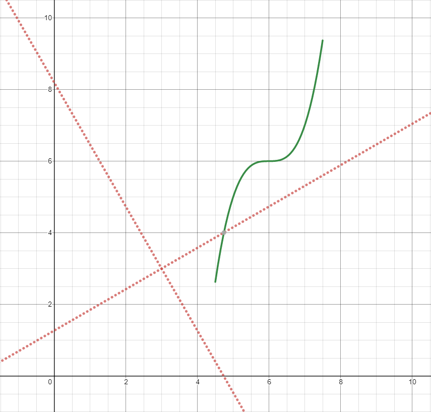
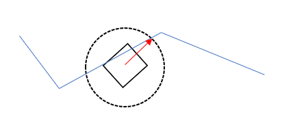
The relativeTo method is used to redefine an already existing trajectory in another frame of reference. This method takes one argument: a pose, (via a Pose2d object) that is defined with respect to the current coordinate system, that represents the origin of the new coordinate system.

For example, a trajectory defined in coordinate system A can be redefined in coordinate system B, whose origin is at (2, 2, 30 degrees) in coordinate system A, using the relativeTo method.

Pose2d bOrigin = new Pose2d(2, 2, Rotation2d.fromDegrees(30));
Trajectory bTrajectory = aTrajectory.relativeTo(bOrigin);

In the diagram above, the original trajectory (aTrajectory in the code above) has been defined in coordinate system A, represented by the black axes. The red axes, located at (2, 2) and 30° with respect to the original coordinate system, represent coordinate system B. Calling relativeTo on aTrajectory will redefine all poses in the trajectory to be relative to coordinate system B (red axes).

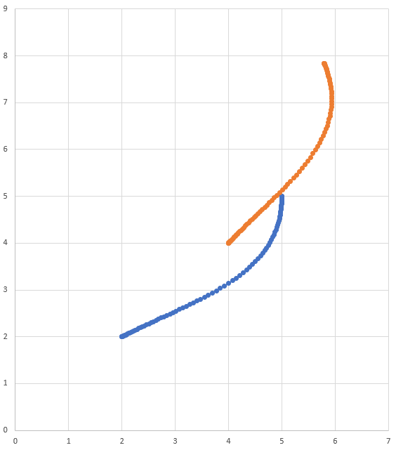
The transformBy Method

The transformBy method can be used to move (i.e. translate and rotate) a trajectory within a coordinate system. This method takes one argument: a transform (via a Transform2d object) that maps the current initial position of the trajectory to a desired initial position of the same trajectory.

For example, one may want to transform a trajectory that begins at (2, 2, 30 degrees) to make it begin at (4, 4, 50 degrees) using the transformBy method.

Transform2d transform = new Pose2d(4, 4, Rotation2d.fromDegrees(50)).minus(trajectory.getInitialPose());
Trajectory newTrajectory = trajectory.transformBy(transform);

In the diagram above, the original trajectory, which starts at (2, 2) and at 30° is visible in blue. After applying the transform above, the resultant trajectory’s starting location is changed to (4, 4) at 50°. The resultant trajectory is visible in orange.

1. Installing from FTCLib

build.gradle

The first thing you need to change from FTCLib is the dependency in build.gradle

Or, if you are using pedroPathing, change to this dependency block

The latest version numbers (as well as a list of all version numbers) are available at:

• Latest core version:

• Latest pedroPathing version:

Please note that you should not and cannot have both FTCLib and SolversLib installed at the same time.

Repositories:

Then, follow the steps in the section. Then follow the final step below (changing imports).

Changing Imports:

Lastly, follow the steps in the section and then Gradle Sync!

2. Installing from SolversLib Quickstart

An alternative option is to simply use the SolversLib Quickstart. Similar to the FTCLib Quickstart, SolversLib has a Quickstart with this library fully set up. You can view it at . You can either fork or clone this repository as needed to use it.

In addition, the Quickstart also has the Pedro Pathing library installed and added along with the SolversLib pedroPathing dependency, meaning that it is hassle-free. If you don't want the Pedro Pathing part, you can simply delete the relevant files.

3. Installing from Scratch

build.common.gradle

First, you need to add the mavenCentral library repository to your build.gradle file at the project root:

Next, minSdkVersion to 24 and multiDexEnabled to true:

Next, change JavaVersion to 8 :

build.gradle (TeamCode)

Add this dependency block for the base library:

The latest version numbers (as well as a list of all version numbers) are available at:

• Latest core version:

• Latest pedroPathing version:

Snapshot Versions

SolversLib is graciously hosted on the Dairy Foundation (thanks to Oscar!), and has release versions and snapshots versions.

• Release versions:

  • Are official, verified versions of SolversLibs

  • Less likelier to have problems/bugs

  • Are in the form: implementation "org.solverslib:core:x.y.z" (where x, y, and z are version numbers).

• Snapshots versions:

  • Are unofficial, and effectively beta versions with newere features and additions

  • More likelier to have problems/bugs

  • Are in the form: implementation "org.solverslib:pedroPathing:SNAPSHOT-abc1234" (7 random letters & numbers).

For most people, it is HIGHLY recommended to use the releases versions. Should you still want to use the snapshots versions instead of releases, you can use the dependencies instead:

• Latest core snapshot version:

• Latest pedroPathing snapshot version:

Repositories:

Look at the section below. Make sure to follow the snapshot versions part.

Repositories

In your repositories block, add the following code. You may have other content here, especially if you have the Pedro Pathing library installed. If you do not have a repositories block, you can add it above your dependencies block.

Only for Snapshot Versions

You also need to add the maven for snapshots in your repositories block in addition to the releases one. Again, if you do not have a repositories block, you can add it above your dependencies block.

Changing Imports

Because the package names will be different, you can either manually replace all instances of com.arcrobotics.ftclib with com.seattlesolvers.solverslib , or use a command in a terminal to replace them all at once for you. Please make sure you either open a terminal into your Android Studio project or use the built-in Android Studio terminal to run the commands below.

FTCLib Imports to SolversLib Imports (MacOS/Linux):

SolversLib Imports to FTCLib Imports (MacOS/Linux):

FTCLib Imports to SolversLib Imports (Windows):

SolversLib Imports to FTCLib Imports (Windows):

Sync Gradle and Finished!

The current command system for SolversLib is modeled closely after that of . Some of the following information may be copied from the source material.

The command-based paradigm is one that allows programming to follow a set design pattern. The specific command system that SolversLib uses follows a declarative programming style. The emphasis is, instead, on what the program should do rather than how to do it. This minimizes the iteration-by-iteration robot logic needed to write out a certain action. Very simply, you can bind some actions to buttons/triggers such as the example below:

Or, instead of binding to a button, you can simply schedule an action to occur by registering it.

Terminology

Let's discuss some of the basic terminology for the paradigm.

Subsystem

A subsystem is the basic unit of robot organization in the design-based paradigm. Subsystems lower-level robot hardware (such as motor controllers, sensors, and/or pneumatic actuators), and define the interfaces through which that hardware can be accessed by the rest of the robot code. Subsystems allow users to “hide” the internal complexity of their actual hardware from the rest of their code - this both simplifies the rest of the robot code, and allows changes to the internal details of a subsystem without also changing the rest of the robot code. Subsystems implement the Subsystem interface.

Command

A command defines high-level robot actions or behaviors that utilize the methods defined by the subsystems. A command is a simple that is either initializing, executing, ending, or idle. Users write code specifying which action should be taken in each state. Simple commands can be composed into “command groups” to accomplish more-complicated tasks. Commands, including command groups, implement the Command interface.

How Commands Are Run

For a more detailed explanation, please see the .

Commands are run by the CommandScheduler, which is a singleton at the base of the command system. The command scheduler is in charge of polling buttons for new commands to schedule, checking the resources required by those commands to avoid conflicts, executing currently-scheduled commands, and removing commands that have finished or been interrupted. The scheduler’s run() method may be called from any place in the user’s code.

Multiple commands can run concurrently, as long as they do not require the same resources on the robot. Resource management is handled on a per-subsystem basis: commands may specify which subsystems they interact with, and the scheduler will never schedule more than one command requiring a given subsystem at a time. This ensures that, for example, users will not end up with two different pieces of code attempting to set the same motor controller to different output values. If a new command is scheduled that requires a subsystem that is already in use, it will either interrupt the currently-running command that requires that subsystem (if the command has been scheduled as interruptible), or else it will not be scheduled.

Subsystems also can be associated with “default commands” that will be automatically scheduled when no other command is currently using the subsystem. This is useful for continuous “background” actions such as controlling the robot drive, or keeping an arm held at a setpoint.

When a command is scheduled, its initialize() method is called once. Its execute() method is then called once per call to CommandScheduler.getInstance().run(). A command is unscheduled and has its end(boolean interrupted) method called when either its isFinished() method returns true, or else it is interrupted (either by another command with which it shares a required subsystem, or by being canceled).

Command Groups

It is often desirable to build complex commands from simple pieces. This is achievable by commands into “command groups.” A is a command that contains multiple commands within it, which run either in parallel or in sequence. The command-based library provides several types of command groups for teams to use, and users are encouraged to write their own, if desired. As command groups themselves implement the Command interface, they are - one can include command groups within other command groups. This provides an extremely powerful way of building complex robot actions with a simple library.

The DifferentialDriveKinematics class is a useful tool that converts between a ChassisSpeeds object and a DifferentialDriveWheelSpeeds object, which contains velocities for the left and right sides of a differential drive robot.

Constructing the Kinematics Object

The DifferentialDriveKinematics object accepts one constructor argument, which is the trackwidth of the robot. This represents the distance between the two sets of wheels on a differential drive.

Note: The trackwidth must be in meters.

Converting Chassis Speeds to Wheel Speeds

The toWheelSpeeds(ChassisSpeeds speeds) method should be used to convert a ChassisSpeeds object to a DifferentialDriveWheelSpeeds object. This is useful in situations where you have to convert a linear velocity (vx) and an angular velocity (omega) to left and right wheel velocities.

Converting Wheel Speeds to Chassis Speeds

One can also use the kinematics object to convert individual wheel speeds (left and right) to a singular ChassisSpeeds object. The toChassisSpeeds(DifferentialDriveWheelSpeeds speeds) method should be used to achieve this.

In the , you might have noticed that no custom constraints were added when generating the trajectories. Custom constraints allow users to impose more restrictions on the velocity and acceleration at points along the trajectory based on location and curvature.

For example, a custom constraint can keep the velocity of the trajectory under a certain threshold in a certain region or slow down the robot near turns for stability purposes.

Provided Constraints

SolversLib includes a set of predefined constraints that users can utilize when generating trajectories. The list of SolversLib-provided constraints is as follows:

• CentripetalAccelerationConstraint: Limits the centripetal acceleration of the robot as it traverses along the trajectory. This can help slow down the robot around tight turns.

• DifferentialDriveKinematicsConstraint: Limits the velocity of the robot around turns such that no wheel of a differential-drive robot goes over a specified maximum velocity.

• DifferentialDriveVoltageConstraint: Limits the acceleration of a differential drive robot such that no commanded voltage goes over a specified maximum.

• MecanumDriveKinematicsConstraint: Limits the velocity of the robot around turns such that no wheel of a -drive robot goes over a specified maximum velocity.

• SwerveDriveKinematicsConstraint: Limits the velocity of the robot around turns such that no wheel of a swerve-drive robot goes over a specified maximum velocity.

Note

The DifferentialDriveVoltageConstraint only ensures that theoretical voltage commands do not go over the specified maximum using a . If the robot were to deviate from the reference while tracking, the commanded voltage may be higher than the specified maximum.

Creating a Custom Constraint

Users can create their own constraint by implementing the TrajectoryConstraint .

The MaxVelocity method should return the maximum allowed velocity for the given pose, curvature, and original velocity of the trajectory without any constraints. The MinMaxAcceleration method should return the minimum and maximum allowed acceleration for the given pose, curvature, and constrained velocity.

A user can use the swerve drive kinematics classes in order to perform . WPILib/SolversLib contains a SwerveDriveOdometry class that can be used to track the position of a swerve drive robot on the field.

Note: Because this method only uses encoders and a gyro, the estimate of the robot’s position on the field will drift over time, especially as your robot comes into contact with other robots during gameplay. However, odometry is usually very accurate during the autonomous period.

Creating the Odometry Object

The SwerveDriveOdometry class requires two mandatory arguments, and one optional argument. The mandatory arguments are the kinematics object that represents your swerve drive (in the form of a SwerveDriveKinematics class) and the angle reported by your gyroscope (as a Rotation2d). The third optional argument is the starting pose of your robot on the field (as a Pose2d). By default, the robot will start at .

0 degrees / radians represents the robot angle when the robot is facing directly toward your opponent’s alliance station. As your robot turns to the left, your gyroscope angle should increase.

Updating the Robot Pose

The update method of the odometry class updates the robot position on the field. The update method takes in the gyro angle of the robot, along with a series of module states (speeds and angles) in the form of a SwerveModuleState each. It is important that the order in which you pass the SwerveModuleState objects is the same as the order in which you created the kinematics object.

This update method must be called periodically, preferably in the periodic() method of a . The update method returns the new updated pose of the robot.

Resetting the Robot Pose

The robot pose can be reset via the resetPose method. This method accepts two arguments – the new field-relative pose and the current gyro angle.

If at any time, you decide to reset your gyroscope, the resetPose method MUST be called with the new gyro angle.

The implementation of getState() above is left to the user. The idea is to get the module state (speed and angle) from each module.

In addition, the getPoseMeters() method can be used to retrieve the current robot pose without an update.

The MecanumDriveKinematics class is a useful tool that converts between a ChassisSpeeds object and a MecanumDriveWheelSpeeds object, which contains velocities for each of the four wheels on a mecanum drive.

Constructing the Kinematics Object

The MecanumDriveKinematics class accepts four constructor arguments, with each argument being the location of a wheel relative to the robot center (as a Translation2d). The order for the arguments is front left, front right, back left, and back right. The locations for the wheels must be relative to the center of the robot. Positive x values represent moving toward the front of the robot whereas positive y values represent moving toward the left of the robot.

// Locations of the wheels relative to the robot center.
Translation2d m_frontLeftLocation =
  new Translation2d(0.381, 0.381);
Translation2d m_frontRightLocation =
  new Translation2d(0.381, -0.381);
Translation2d m_backLeftLocation =
  new Translation2d(-0.381, 0.381);
Translation2d m_backRightLocation =
  new Translation2d(-0.381, -0.381);

// Creating my kinematics object using the wheel locations.
MecanumDriveKinematics m_kinematics = new MecanumDriveKinematics
(
  m_frontLeftLocation, m_frontRightLocation,
  m_backLeftLocation, m_backRightLocation
);

Converting Chassis Speeds to Wheel Speeds

The toWheelSpeeds(ChassisSpeeds speeds) method should be used to convert a ChassisSpeeds object to a MecanumDriveWheelSpeeds object. This is useful in situations where you have to convert a forward velocity, sideways velocity, and an angular velocity into individual wheel speeds.

// Example chassis speeds: 1 meter per second forward, 3 meters
// per second to the left, and rotation at 1.5 radians per second
// counterclockwise.
ChassisSpeeds speeds = new ChassisSpeeds(1.0, 3.0, 1.5);

// Convert to wheel speeds
MecanumDriveWheelSpeeds wheelSpeeds =
    kinematics.toWheelSpeeds(speeds);

// Get the individual wheel speeds
double frontLeft = wheelSpeeds.frontLeftMetersPerSecond;
double frontRight = wheelSpeeds.frontRightMetersPerSecond;
double backLeft = wheelSpeeds.rearLeftMetersPerSecond;
double backRight = wheelSpeeds.rearRightMetersPerSecond;

Field-Oriented Drive

Recall that a ChassisSpeeds object can be created from a set of desired field-oriented speeds. This feature can be used to get wheel speeds from a set of desired field-oriented speeds.

// The desired field relative speed here is 2 meters per second
// toward the opponent's alliance station wall, and 2 meters per
// second toward the left field boundary. The desired rotation
// is a quarter of a rotation per second counterclockwise.
// The current robot angle is 45 degrees.
ChassisSpeeds speeds = ChassisSpeeds.fromFieldRelativeSpeeds(
  2.0, 2.0, Math.PI / 2.0, Rotation2d.fromDegrees(45.0)
);

// Now use this in our kinematics
MecanumDriveWheelSpeeds wheelSpeeds =
  kinematics.toWheelSpeeds(speeds);

Using Custom Centers of Rotation

Sometimes, rotating around one specific corner might be desirable for certain evasive maneuvers. This type of behavior is also supported by the WPILib classes. The same toWheelSpeeds() method accepts a second parameter for the center of rotation (as a Translation2d). Just like the wheel locations, the Translation2d representing the center of rotation should be relative to the robot center.

Because all robots are a rigid frame, the provided vx and vy velocities from the ChassisSpeeds object will still apply for the entirety of the robot. However, the omega from the ChassisSpeeds object will be measured from the center of rotation.

For example, one can set the center of rotation on a certain wheel and if the provided ChassisSpeeds object has a vx and vy of zero and a non-zero omega, the robot will appear to rotate around that particular wheel.

Converting Wheel Speeds to Chassis speeds

One can also use the kinematics object to convert a MecanumDriveWheelSpeeds object to a singular ChassisSpeeds object. The toChassisSpeeds(MecanumDriveWheelSpeeds speeds) method can be used to achieve this.

// Example wheel speeds
MecanumDriveWheelSpeeds wheelSpeeds =
    new MecanumDriveWheelSpeeds(-17.67, 20.51, -13.44, 16.26);

// Convert to chassis speeds
ChassisSpeeds chassisSpeeds =
    kinematics.toChassisSpeeds(wheelSpeeds);

// Getting individual speeds
double forward = chassisSpeeds.vxMetersPerSecond;
double sideways = chassisSpeeds.vyMetersPerSecond;
double angular = chassisSpeeds.omegaRadiansPerSecond;

Subsystems are the basic unit of robot organization in the command-based paradigm. A subsystem is an abstraction for a collection of robot hardware that operates together as a unit. Subsystems encapsulate this hardware, “hiding” it from the rest of the robot code (e.g. commands) and restricting access to it except through the subsystem’s public methods. Restricting the access in this way provides a single convenient place for code that might otherwise be duplicated in multiple places (such as scaling motor outputs or checking limit switches) if the subsystem internals were exposed. It also allows changes to the specific details of how the subsystem works (the “implementation”) to be isolated from the rest of robot code, making it far easier to make substantial changes if/when the design constraints change.

Subsystems also serve as the backbone of the CommandScheduler’s resource management system. Commands may declare resource requirements by specifying which subsystems they interact with; the scheduler will never concurrently schedule more than one command that requires a given subsystem. An attempt to schedule a command that requires a subsystem that is already-in-use will either interrupt the currently-running command (if the command has been scheduled as interruptible), or else be ignored.

Subsystems can be associated with “default commands” that will be automatically scheduled when no other command is currently using the subsystem. This is useful for continuous “background” actions such as controlling the robot drive, or keeping an arm held at a setpoint. Similar functionality can be achieved in the subsystem’s periodic() method, which is run once per run of the scheduler; teams should try to be consistent within their codebase about which functionality is achieved through either of these methods. Subsystems are represented in the command-based library by the Subsystem interface.

Creating a Subsystem

The recommended method to create a subsystem for most users is to subclass the abstract SubsystemBase class, as seen in the command-based template:

import com.seattlesolvers.solverslib.command.SubsystemBase;

public class ExampleSubsystem extends SubsystemBase {
  /**
   * Creates a new ExampleSubsystem.
   */
  public ExampleSubsystem() {

  }

  @Override
  public void periodic() {
    // This method will be called once per scheduler run
  }
}

This class contains automatically calls the register() method in its constructor to register the subsystem with the scheduler (this is necessary for the periodic() method to be called when the scheduler runs).

Advanced users seeking more flexibility may simply create a class that implements the Subsystem interface.

Creating a Simple Subsystem

Subsystems are easy to create. They combine different sets of hardware to produce either multiple or one particular task. Hence why they are the basic unit of organization in the command system. Below is a simple example:

package org.firstinspires.ftc.robotcontroller.external.samples.CommandSample;

import com.seattlesolvers.solverslib..command.SubsystemBase;
import com.qualcomm.robotcore.hardware.HardwareMap;
import com.qualcomm.robotcore.hardware.Servo;

/**
 * A gripper mechanism that grabs a stone from the quarry.
 * Centered around the Skystone game for FTC that was done in the 2019
 * to 2020 season.
 */
public class GripperSubsystem extends SubsystemBase {

    private final Servo mechRotation;

    public GripperSubsystem(final HardwareMap hMap, final String name) {
        mechRotation = hMap.get(Servo.class, name);
    }

    /**
     * Grabs a stone.
     */
    public void grab() {
        mechRotation.setPosition(0.76);
    }

    /**
     * Releases a stone.
     */
    public void release() {
        mechRotation.setPosition(0);
    }

}

Setting Default Commands

“Default commands” are commands that run automatically whenever a subsystem is not being used by another command.

Setting a default command for a subsystem is very easy; one simply calls CommandScheduler.getInstance().setDefaultCommand(), or, more simply, the setDefaultCommand() method of the Subsystem interface which can be called in the OpMode:

CommandScheduler.getInstance().setDefaultCommand(exampleSubsystem, exampleCommand);

exampleSubsystem.setDefaultCommand(exampleCommand);

A user can use the mecanum drive kinematics classes in order to perform odometry. WPILib/SolversLib contains a MecanumDriveOdometry class that can be used to track the position of a mecanum drive robot on the field.

Note: Because this method only uses encoders and a gyro, the estimate of the robot’s position on the field will drift over time, especially as your robot comes into contact with other robots during gameplay. However, odometry is usually very accurate during the autonomous period.

Creating the Odometry Object

The MecanumDriveOdometry class requires two mandatory arguments and one optional argument. The mandatory arguments are the kinematics object that represents your mecanum drive (in the form of a MecanumDriveKinematics class) and the angle reported by your gyroscope (as a Rotation2d). The third optional argument is the starting pose of your robot on the field (as a Pose2d). By default, the robot will start at $\begin{pmatrix} x\\ y\\ \theta \end{pmatrix} = \begin{pmatrix} 0\\ 0\\ 0 \end{pmatrix}$ .

0 degrees / radians represents the robot angle when the robot is facing directly toward your opponent’s alliance station. As your robot turns to the left, your gyroscope angle should increase.

// Locations of the wheels relative to the robot center.
Translation2d m_frontLeftLocation =
  new Translation2d(0.381, 0.381);
Translation2d m_frontRightLocation =
  new Translation2d(0.381, -0.381);
Translation2d m_backLeftLocation =
  new Translation2d(-0.381, 0.381);
Translation2d m_backRightLocation =
  new Translation2d(-0.381, -0.381);

// Creating my kinematics object using the wheel locations.
MecanumDriveKinematics m_kinematics = new MecanumDriveKinematics
(
  m_frontLeftLocation, m_frontRightLocation,
  m_backLeftLocation, m_backRightLocation
);

// Creating my odometry object from the kinematics object. Here,
// our starting pose is 5 meters along the long end of the field and in the
// center of the field along the short end, facing forward.
MecanumDriveOdometry m_odometry = new MecanumDriveOdometry
(
  m_kinematics, getGyroHeading(),
  new Pose2d(5.0, 13.5, new Rotation2d()
);

Updating the Robot Pose

The update method of the odometry class updates the robot position on the field. The update method takes in the gyro angle of the robot, along with a MecanumDriveWheelSpeeds object representing the speed of each of the 4 wheels on the robot. This update method must be called periodically, preferably in the periodic() method of a Subsystem. The update method returns the new updated pose of the robot.

The MecanumDriveWheelSpeeds class must be constructed with each wheel speed in meters per second.

@Override
public void periodic() {
  // Get my wheel speeds; assume .getRate() has been
  // set up to return velocity of the encoder
  // in meters per second.
  MecanumDriveWheelSpeeds wheelSpeeds = new MecanumDriveWheelSpeeds
  (
      m_frontLeftEncoder.getRate(), m_frontRightEncoder.getRate(),
      m_backLeftEncoder.getRate(), m_backRightEncoder.getRate()
  );

  // Get my gyro angle.
  Rotation2d gyroAngle = Rotation2d.fromDegrees(m_gyro.getAngle());

  // Update the pose
  m_pose = m_odometry.update(gyroAngle, wheelSpeeds);
}

Resetting the Robot Pose

The robot pose can be reset via the resetPose method. This method accepts two arguments – the new field-relative pose and the current gyro angle.

If at any time, you decide to reset your gyroscope, the resetPose method MUST be called with the new gyro angle.

In addition, the getPoseMeters() method can be used to retrieve the current robot pose without an update.

SolversLib offers its own odometry classes for the use of differential and holonomic drives. The odometry classes track the robot position as a Pose2d, which means it is represented using the vector . is the distance in the forward direction of the robot, is the horizontal distance, and is the heading of the robot.

When using these classes, it is important to keep angles in radians. Distances should be consistent.

Pose Exponential

Pose Exponential is a general FRC term for the constant velocity method of odometry utilized in FTC. We use pose exponentials because the cycle times of control loops in FTC can vary significantly.

This method uses differential equations to solve the nonlinear position of the robot given constant curvature. As such, we will not explain the math here. If you are interested in the math behind it, we suggest you read up on .

Offsets and Trackwidth

The trackwidth is the distance between parallel encoders. This value should be tuned so that a precise calculation can be made. This value is a required pass into the constructor.

The center wheel offset accounts for the distance between the center of rotation of the robot and the position of the horizontal encoder. This is only necessary for the holonomic odometry.

To tune these values, make a rough estimate with a measured value and then use some sort of method for testing and updating the values until the outputs become reliable. Alternatively to beginning with a measured value, you can start at 18. Your value should then converge to some smaller distance.

Creating the Odometry

A sample usage of SolversLib odometry can be found in this . A sample for dead wheels can be found .

Using the Odometry Class

To use the odometry class, there are three different constructors depending on how you want to run your odometry. One method of running the odometry is using suppliers to have the class update your positions for you. The other is to manually input the sensor data into the update() method, which has parameters of the left encoder value, right encoder value, and horizontal encoder value (which is only used for holonomic). If you use suppliers, you can just call the updatePose() method which uses the suppliers to call the update() method.

You should call the respective update method once every cycle of the control loop.

Using the Odometry Subsystem

The class is a template subsystem meant to make command-based programming around odometry much simpler and functional. Using the odometry subsystem makes it more accurate because the position will update itself through the scheduler's call to its periodic() method, which updates the position. The subsystem makes use of the suppliers, so you will need to use that constructor instead of the other for the SolversLib subsystem. Alternatively, you can create your own odometry subsystem.

The makes use of the OdometrySubsystem class.

This article goes over how to generate a trajectory. The next few articles in this series will go over how to actually follow the generated trajectory. There are a few things that your robot must have before you dive into the world of trajectories:

• A way to measure the position and velocity of each side of the robot. An encoder is the best way to do this; however, other options may include optical flow sensors, etc.

• A way to measure the angle or angular rate of the robot chassis. A gyroscope is the best way to do this. Although the angular rate can be calculated using encoder velocities, this method is NOT recommended because of wheel scrubbing.

Splines

A refers to a set of curves that interpolate between points. Think of it as connecting dots, except with curves. SolversLib supports two types of splines: hermite clamped cubic and hermite quintic.

• Hermite clamped cubic: This is the recommended option for most users. Generation of trajectories using these splines involves specifying the (x, y) coordinates of all points, and the headings at the start and end waypoints. The headings at the interior waypoints are automatically determined to ensure continuous curvature (rate of change of the heading) throughout.

• Hermite quintic: This is a more advanced option which requires the user to specify (x, y) coordinates and headings for all waypoints. This should be used if you are unhappy with the trajectories that are being generated by the clamped cubic splines or if you want finer control of headings at the interior points.

Splines are used as a tool to generate trajectories; however, the spline itself does not have any information about velocities and accelerations. Therefore, it is not recommended that you use the spline classes directly. In order to generate a smooth path with velocities and accelerations, a trajectory must be generated.

Creating the Trajectory Configuration

A configuration must be created in order to generate a trajectory. The config contains information about special constraints, the max velocity, the max acceleration in addition to the start velocity and end velocity. The config also contains information about whether the trajectory should be reversed (robot travels backward along the waypoints). The TrajectoryConfig class should be used to construct a config. The constructor for this class takes two arguments, the max velocity and max acceleration. The other fields (startVelocity, endVelocity, reversed, constraints) are defaulted to reasonable values (0, 0, false, {}) when the object is created. If you wish to modify the values of any of these fields, you can call the following methods:

• setStartVelocity(double startVelocityMetersPerSecond)

• setEndVelocity(double endVelocityMetersPerSecond)

• setReversed(boolean reversed)

• addConstraint(TrajectoryConstraint constraint)

NOTE

The reversed property simply represents whether the robot is traveling backward. If you specify four waypoints, a, b, c, and d, the robot will still travel in the same order through the waypoints when the reversed flag is set to true. This also means that you must account for the direction of the robot when providing the waypoints. For example, if your robot is facing your alliance station wall and travels backwards to some field element, the starting waypoint should have a rotation of 180 degrees.

Generating the Trajectory

The method used to generate a trajectory is generateTrajectory(...). There are four overloads for this method. Two that use clamped cubic splines and the two others that use quintic splines. For each type of spline, there are two ways to construct a trajectory. The easiest methods are the overloads that accept Pose2d objects.

For clamped cubic splines, this method accepts two Pose2d objects, one for the starting waypoint and one for the ending waypoint. The method takes in a vector of Translation2d objects which represent the interior waypoints. The headings at these interior waypoints are determined automatically to ensure continuous curvature. For quintic splines, the method simply takes in a list of Pose2d objects, with each Pose2d representing a point and heading on the field.

The more complex overload accepts “control vectors” for splines. The ControlVector class consists of two double arrays. Each array represents one dimension (x or y), and its elements represent the derivatives at that point. For example, the value at element 0 of the x array represents the x coordinate (0th derivative), the value at element 1 represents the 1st derivative in the x dimension and so on.

When using clamped cubic splines, the length of the array must be 2 (0th and 1st derivatives), whereas when using quintic splines, the length of the array should be 3 (0th, 1st, and 2nd derivative). Unless you know exactly what you are doing, the first and simpler method is HIGHLY recommended for manually generating trajectories.

Here is an example of generating a trajectory using clamped cubic splines for the 2018 game, FIRST Power Up:

Note that this is not code from SolversLib and is instead a sample from WPILib docs. The keyword var is used here, but that is a feature from Java 10 which is not supported for Android development. The keyword has the compiler interpret the variable type and assign accordingly. Instead of this, use the actual variable type definition. The Units class is also not available in SolversLib and is instead a WPILib utility.

NOTE: We recommend using the for your implementation of the command-based paradigm as it is much friendlier for FTC programs.

The Robot Class

The class makes using the CommandScheduler so much simpler in the user's code. Similar to WPILib, the Robot class allows for making a Robot paradigm. This allows for the creation of multiple opmodes tied to one object. This is also the basis for disabling the robot, meaning we want to interrupt the commands and not allow for scheduling new ones. This is done with the static disable() and enable() methods:

Creating a Robot Class

The first step in using the Robot paradigm is to create your own Robot subclass. This will maintain all of the commands and subsystems you want to utilize. Also note that you can schedule and register new commands and subsystems from outside the Robot class using the schedule() and register() methods.

A major downside of the Robot class is that it shares the common commands and subsystems for every use in the OpModes. A recommendation is to create an inside of your robot implementation that specifies TeleOp versus Autonomous so that when the object is constructed, it uses the desired CommandScheduler instance.

Below is an example of utilizing this feature.

A downside that cannot be fixed by this is when you want to run several different opmodes of the different types with respect to the same subsystems. This is where the comes in handy and makes the paradigm a lot more FTC-friendly.

Running the Robot in Your OpMode

Running the robot in the opmode is simple and only requires a few lines of code and making a call to the run() method.

CommandOpMode

The is the center of the FTC-centric command-based paradigm. It makes everything simpler for the user and greatly decreases the amount of code needed to run everything. Unlike the Robot class, it is opmode-specific, so it does not store a common reference to subsystems. If desired, the user can create a map that houses all of the referenced hardware, but this is currently not a feature offered (but totally supported) by SolversLib.

If desired, the user can override the methods from the CommandOpMode. Similarly to the Robot class, you can disable the CommandOpMode with static methods (which actually disable the Robot class, which is what is referenced in the CommandScheduler for runsWhenDisabled() commands.

Initializing your Hardware

CommandOpMode is an abstract class, which means the user must create their own implementation of it. The only method that needs to be implemented is the initialize() method, which instantiates all of the hardware and commands to be run by the scheduler. The CommandOpMode class already implements the runOpMode() method and runs the scheduler. After the opmode is no longer active or a stop is requested, it resets the instance of the scheduler so a new opmode can be run with a fresh instance. This is very nonintuitive, but it works as designed (setting the singleton instance to null, where a new instance is then created upon calling getInstance().

That is functionally all that needs to be done, everything else is done for the user internally. You can find a sample project utilizing CommandOpMode .

Please note that the following is deprecated. Refer to the new commands if you want to make use of the new paradigm.

SolversLib provides a Command-based OpMode to define your robot's OpMode routine. Instead of hard-coding instructions in your OpMode, you can leverage the reusability of the CommandOpMode structure to predefined Command routines and run them sequentially. You can also set timeouts for a Command to automatically terminate a running command.

Subsystem

Defines an organized module on your robot. One such example is a linear slide lift powered by a motor connected to a spool, additionally using encoders or touch/magnetic sensors to act as limit switches, preventing the lift from exceeding its bounds. In this example, the motor, its encoder, and any sensors used would fall under a single "Lift" Subsystem.

A Subsystem has five lifecycle phases:

• initialize(): Prepares the physical hardware for activation of the Subsystem. This phase is intended to be used for hardware map initialization, zeroing of encoders (as required), and gathering any initially required sensor data.

• reset(): Returns the Subsystem back to its original state. This phase is distinct from initialize() as it is expected that the hardware map is already initialized. This phase is intended to return Subsystem hardware to its original condition and clear saved data.

• loop(): This is the main lifecycle phase of a Subsystem. This is where could be issued to the Subsystem, or user/sensor input is used to operate the Subsystem. This phase is intended to repeatedly loop until stop() is called.

• stop(): Halts all action of the Subsystem, bringing all hardware devices to stop. It is recommended to set the Zero Power Behavior of Motors to BRAKE in this phase, as motion is designed to entirely cease. A Subsystem should be designed to enable a reset() from this phase to return it to normal operation.

• disable(): Deactivates the Subsystem, rendering it unusable until the next initialize(). It is recommended to set the Zero Power Behavior of Motors to FLOAT in this phase, as Subsystem will no longer be receiving input. A Subsystem should NOT be designed to enable reset(), initialize() is required.

Command

Defines a single, executable command. A Command defines the actions of multiples parts (or ) of the robot to take at once. A Command has three lifecycle phases:

• initialize(): The initial subroutine of a Command. Called once when the Command is initially scheduled.

• execute(): The main body of a Command. Called repeatedly while the Command is scheduled.

• end(): The action to take once the Command is completed. Called once on the Command's completion.

Command also provides a isFinished() method which returns true if the Command has completed and false otherwise. Note: end() will always run after the Command is unscheduled. You do not need to check if the Command isFinished() to run your own end() method.

CommandOpMode

Defines an OpMode which is designed to run on as opposed to manual method calls. Before using a CommandOpMode, Commands and need to be defined. CommandOpMode runs an internal ElapsedTimer which ensures Commands terminate after their specified timeouts.

Although CommandOpMode extends LinearOpMode , it is not required to use any of the methods provided explicitly. These methods are all called internally by runOpMode() (it is not necessary to override this method within your own extension of CommandOpMode) within the three lifecycle phases of a CommandOpMode (it is required to override these methods):

• initialize(): Sets up and calls initialize() of all attached Subsystems and Commands. It is vital to setup Subsystems before their Commands, as doing the reverse could likely raise NullPointerExceptions.

• initLoop(): Called repeatedly after initialize() but before the user presses "Play" on the Driver Station

• run(): The main loop of a CommandOpMode. Called immediately after the user presses the "Play" button on the Driver Station.

Internally, these three lifecycle phases are tied together under an override of the runOpMode() method of LinearOpMode:

Once the user defines Commands, Subsystems, and the three lifecycle phases, the user can add Commands to the workflow using addSequential(). addSequential() adds a Command to be run within a certain specified timeout. The user can also optionally set a custom loop interval time (which defaults to 20 ms). addSequential() first initializes its passed-in Command, runs it every 20 ms (terminating if it reaches its timeout), and checks if the Command isFinished(). If true, the Command will exit the loop and run its end() lifecycle method.

Individual commands are capable of accomplishing a large variety of robot tasks, but the simple three-state format can quickly become cumbersome when more advanced functionality requiring extended sequences of robot tasks or coordination of multiple robot subsystems is required. In order to accomplish this, users are encouraged to use the powerful command group functionality included in the command-based library.

As the name suggests, command groups are combinations of multiple commands. The act of combining multiple objects (such as commands) into a bigger object is known as composition. Command groups compose multiple commands into a composite command. This allows code to be kept much cleaner and simpler, as the individual component commands may be written independently of the code that combines them, greatly reducing the amount of complexity at any given step of the process.

Most importantly, however, command groups are themselves commands - they implement the Command interface. This allows command groups to be recursively composed - that is, a command group may contain other command groups as components.

Types of Command Groups

The command-based library supports four basic types of command groups: SequentialCommandGroup, ParallelCommandGroup, ParallelRaceGroup, and ParallelDeadlineGroup. Each of these command groups combines multiple commands into a composite command - however, they do so in different ways:

SequentialCommandGroup

A SequentialCommandGroup runs a list of commands in sequence - the first command will be executed, then the second, then the third, and so on until the list finishes. The sequential group finishes after the last command in the sequence finishes. It is therefore usually important to ensure that each command in the sequence does actually finish (if a given command does not finish, the next command will never start!).

ParallelCommandGroup

A ParallelCommandGroup runs a set of commands concurrently - all commands will execute at the same time. The parallel group will end when all commands have finished.

ParallelRaceGroup

A ParallelRaceGroup is much like a ParallelCommandgroup, in that it runs a set of commands concurrently. However, the race group ends as soon as any command in the group ends - all other commands are interrupted at that point.

ParallelDeadlineGroup

A ParallelDeadlineGroupalso runs a set of commands concurrently. However, the deadline group ends when a specific command (the “deadline”) ends, interrupting all other commands in the group that are still running at that point.

Creating Command Groups

Users have several options for creating command groups. One way - similar to the previous implementation of the command-based library - is to subclass one of the command group classes. Below is an example of a command group:

import com.seattlesolvers.solverslib.command.SequentialCommandGroup;

/**
 * A complex auto command that drives forward,
 * releases a stone, and then drives backward.
 */
public class ReleaseAndBack extends SequentialCommandGroup {

    private static final double INCHES = 3.0;
    private static final double SPEED = 0.5;

    /**
     * Creates a new ReleaseAndBack command group.
     *
     * @param drive The drive subsystem this command will run on
     * @param grip The gripper subsystem this command will run on
     */
    public ReleaseAndBack(DriveSubsystem drive, GripperSubsystem grip)
    {
        addCommands(
                new DriveDistance(INCHES, SPEED, drive),
                new ReleaseStone(grip),
                new DriveDistance(INCHES, SPEED, drive)
        );
        addRequirements(drive, grip);
    }

}

The addCommands() method adds commands to the group, and is present in all four types of command group.

Inline Command Groups

Command groups can be used without subclassing at all: one can simply pass in the desired commands through the constructor:

new SequentialCommandGroup(new FooCommand(), new BarCommand());

This is called an inline command definition, and is very handy for circumstances where command groups are not likely to be reused, and writing an entire class for them would be wasteful.

Recursive Composition of Command Groups

As mentioned earlier, command groups are recursively composable - since command groups are themselves commands, they may be included as components of other command groups. This is an extremely powerful feature of command groups, and allows users to build very complex robot actions from simple pieces. For example, consider the following code:

new SequentialCommandGroup(
   new DriveToGoal(m_drive),
   new ParallelCommandGroup(
      new RaiseElevator(m_elevator),
      new SetWristPosition(m_wrist)),
   new ScoreTube(m_wrist));

Notice how the recursive composition allows the embedding of a parallel control structure within a sequential one. Notice also that this entire, more-complex structure, could be again embedded in another structure. Composition is an extremely powerful tool, and one that users should be sure to use extensively.

Command Group and Requirements

As command groups are commands, they also must declare their requirements. However, users are not required to specify requirements manually for command groups - requirements are automatically inferred from the commands included. As a rule, command groups include the union of all of the subsystems required by their component commands. Thus, the ReleaseAndBack shown previously will require both the drive subsystem and the gripper subsystem of the robot.

Additionally, requirements are enforced within all three types of parallel groups - a parallel group may not contain multiple commands that require the same subsystem.

Some advanced users may find this overly-restrictive - for said users, the library offers a ScheduleCommand class that can be used to independently “branch off” from command groups to provide finer granularity in requirement management.

Restrictions on Command Group Components

Since command group components are run through their encapsulating command groups, errors could occur if those same command instances were independently scheduled at the same time as the group - the command would be being run from multiple places at once, and thus could end up with inconsistent internal state, causing unexpected and hard-to-diagnose behavior.

For this reason, command instances that have been added to a command group cannot be independently scheduled or added to a second command group. Attempting to do so will throw an exception and crash the user program.

Advanced users who wish to re-use a command instance and are certain that it is safe to do so may bypass this restriction with the clearGroupedCommand() method in the CommandGroupBase class.

Apart from autonomous commands, which are scheduled at the start of the autonomous period, and default commands, which are automatically scheduled whenever their subsystem is not currently in-use, the most common way to run a command is by binding it to a triggering event, such as a button being pressed by a human operator. The command-based paradigm makes this extremely easy to do.

As mentioned earlier, command-based is a declarative paradigm. Accordingly, binding buttons to commands is done declaratively; the association of a button and a command is “declared” once, during robot initialization. The library then does all the hard work of checking the button state and scheduling (or cancelling) the command as needed, behind-the-scenes. Users only need to worry about designing their desired UI setup - not about implementing it!

Command binding is done through the Trigger class and its various Button subclasses.

Trigger/Button Bindings

There are a number of bindings available for the Trigger class. All of these bindings will automatically schedule a command when a certain trigger activation event occurs - however, each binding has different specific behavior. Button and its subclasses have bindings with identical behaviors, but slightly different names that better-match a button rather than an arbitrary triggering event.

whenActive/whenPressed

This binding schedules a command when a trigger changes from inactive to active (or, accordingly, when a button changes is initially pressed). The command will be scheduled on the iteration when the state changes, and will not be scheduled again unless the trigger becomes inactive and then active again (or the button is released and then re-pressed).

whileActiveContinuous/whileHeld

This binding schedules a command repeatedly while a trigger is active (or, accordingly, while a button is held), and cancels it when the trigger becomes inactive (or when the button is released). Note that scheduling an already-running command has no effect; but if the command finishes while the trigger is still active, it will be re-scheduled.

whileActiveOnce/whenHeld

This binding schedules a command when a trigger changes from inactive to active (or, accordingly, when a button is initially pressed) and cancels it when the trigger becomes inactive again (or the button is released). The command will not be re-scheduled if it finishes while the trigger is still active.

whenInactive/whenReleased

This binding schedules a command when a trigger changes from active to inactive (or, accordingly, when a button is initially released). The command will be scheduled on the iteration when the state changes, and will not be re-scheduled unless the trigger becomes active and then inactive again (or the button is pressed and then re-released).

toggleWhenActive/toggleWhenPressed

This binding toggles a command, scheduling it when a trigger changes from inactive to active (or a button is initially pressed), and cancelling it under the same condition if the command is currently running. Note that while this functionality is supported, toggles are not a highly-recommended option for user control, as they require the driver to mentally keep track of the robot state.

Since v1.2.0, courtesy of Ethan Leitner, the toggle binding has an additional option of switching between two commands. This is a replacement of the ConditionalCommand option for toggling. Simply pass two commands into the method instead of one, and the binding will toggle between those two commands.

cancelWhenActive/cancelWhenPressed

This binding cancels a command when a trigger changes from inactive to active (or, accordingly, when a button is initially pressed). the command is canceled on the iteration when the state changes, and will not be canceled again unless the trigger becomes inactive and then active again (or the button is released and re-pressed). Note that cancelling a command that is not currently running has no effect.

Binding a Command to a Gamepad Button

The most-common way to trigger a command is to bind a command to a button on the gamepad.

Creating a GamepadButton

In order to create a GamepadButton, we first need a GamepadEx.

GamepadEx driverOp = new GamepadEx(gamepad1);
GamepadEx toolOp = new GamepadEx(gamepad2);

When the object is instantiated, users can then pass it into the GamepadButton class.

Button exampleButton = new GamepadButton(
    driverOp, GamepadKeys.Button.A
);

// alternatively, you can use the mapped GamepadButtons
// built in to the GamepadEx class
driverOp.getGamepadButton(GamepadKeys.Button.A);

Binding a Command to a Button

Putting it all together, it is very simple to bind a command to a Button.

exampleButton.whenPressed(new ExampleCommand());

/* It is super useful to also use instant commands */
exampleButton.whenPressed(new InstantCommand(() -> {
    // your implementation of Runnable.run() here
}));

It is useful to note that the command binding methods all return the trigger/button that they were initially called on, and thus can be chained to bind multiple commands to different states of the same button. For example:

exampleButton
    // Binds a FooCommand to be scheduled when the `X` button
    // of the driver gamepad is pressed
    .whenPressed(new FooCommand())
    // Binds a BarCommand to be scheduled when that same button
    // is released
    .whenReleased(new BarCommand());
    
// instantiation + binding
    
/* You can also do this when you create a button object */
Button exampleButton = new GamepadButton(
    driverOp, GamepadKeys.Button.A
    // then bind commands
).whenPressed(new FooCommand())
    .whenReleased(new BarCommand());
    
/* You can also do this with the GamepadEx button mapping */
driverOp.getGamepadButton(GamepadKeys.Button.A)
    .whenPressed(new FooCommand())
    .whenReleased(new BarCommand());

Remember that button binding is declarative. Bindings only need to be declared once, ideally some time during robot initialization. The library handles everything else.

Composing Triggers

The Trigger class (including its Button subclasses) can be composed to create composite triggers through the and(), or(), and negate() methods. For example:

// Binds an ExampleCommand to be scheduled when both the 'X' and
// 'Y' buttons of the driver gamepad are pressed
new GamepadButton(driverOp, GamepadKeys.Button.X)
    .and(new GamepadButton(exampleController, GamepadKeys.Button.Y))
    .whenActive(new ExampleCommand());

Note that these methods return a Trigger, not a Button, so the Trigger binding method names must be used even when buttons are composed.

Creating Your Own Custom Trigger

While binding to buttons is by far the most common use case, advanced users may occasionally want to bind commands to arbitrary triggering events. This can be easily done by simply writing your own subclass of Trigger or Button:

public class ExampleTrigger extends Trigger {
  @Override
  public boolean get() {
    // This returns whether the trigger is active
  }
}

Alternatively, this can also be done inline by passing a lambda to the constructor of Trigger or Button:

// Here it is assumed that "condition" is an object with a
// method "get" that returns whether the trigger should be active
Trigger exampleTrigger = new Trigger(condition::get);

This can be used for implementing a type of "triggering condition," which one might see with a sensor. On the activation of the trigger, you can cause certain commands to be scheduled or cancelled.

Commands are simple state machines that perform high-level robot functions using the methods defined by subsystems. Commands can be either idle, in which they do nothing, or scheduled, in which the scheduler will execute a specific set of the command’s code depending on the state of the command. The CommandScheduler recognizes scheduled commands as being in one of three states: initializing, executing, or ending. Commands specify what is done in each of these states through the initialize(), execute() and end() methods. Commands are represented in the command-based library by the Command interface.

Creating Commands

Similarly to subsystems, the recommended method for most users to create a command is to subclass the abstract CommandBase class, as seen in the command-based template.

import com.seattlesolvers.solverslib.command.CommandBase;

/**
 * An example command that uses an example subsystem.
 */
public class ExampleCommand extends CommandBase {
  @SuppressWarnings({"PMD.UnusedPrivateField", "PMD.SingularField"})
  private final ExampleSubsystem m_subsystem;

  /**
   * Creates a new ExampleCommand.
   *
   * @param subsystem The subsystem used by this command.
   */
  public ExampleCommand(ExampleSubsystem subsystem) {
    m_subsystem = subsystem;
    // Use addRequirements() here to declare subsystem dependencies.
    addRequirements(subsystem);
  }
}

As before, this contains several convenience features. It automatically overrides the getRequirements() method for users, returning a list of requirements that is empty by default, but can be added to with the addRequirements() method.

Also as before, advanced users seeking more flexibility are free to simply create their own class implementing the Command interface.

To schedule a command to the scheduler, you will need to call the schedule() method of the command instance.

m_command.schedule();

To schedule a command as uninterruptible, you can simply schedule it as false. The default schedule is true (interruptible).

m_command.schedule(false);

The Structure of a Command

While subsystems are fairly freeform, and may generally look like whatever the user wishes them to, commands are quite a bit more constrained. Command code must specify what the command will do in each of its possible states. This is done by overriding the initialize(), execute(), and end() methods. Additionally, a command must be able to tell the scheduler when (if ever) it has finished execution - this is done by overriding the isFinished() method. All of these methods are defaulted to reduce clutter in user code: initialize(), execute(), and end() are defaulted to simply do nothing, while isFinished() is defaulted to return false (resulting in a command that never ends).

Initialization

The initialize() method is run exactly once per time a command is scheduled, as part of the scheduler’s schedule() method. The scheduler’s run() method does not need to be called for the initialize() method to run. The initialize block should be used to place the command in a known starting state for execution. It is also useful for performing tasks that only need to be performed once per time scheduled, such as setting motors to run at a constant speed.

Execution

The execute() method is called repeatedly while the command is scheduled, whenever the scheduler’s run() method is called. The execute block should be used for any task that needs to be done continually while the command is scheduled, such as updating motor outputs to match joystick inputs, or using the output of a control loop.

Ending

The end() method is called once when the command ends, whether it finishes normally (i.e. isFinished() returned true) or it was interrupted (either by another command or by being explicitly canceled). The method argument specifies the manner in which the command ended; users can use this to differentiate the behavior of their command end accordingly. The end block should be used to “wrap up” command state in a neat way, such as setting motors back to zero or reverting a solenoid actuator to a “default” state.

Specifying End Conditions

The isFinished() method is called repeatedly while the command is scheduled, whenever the scheduler’s run() method is called. As soon as it returns true, the command’s end() method is called and it is unscheduled. The isFinished() method is called after the execute() method, so the command will execute once on the same iteration that it is unscheduled.

Simple Command Example

Taking the gripper example from the Subsystem page, we can develop the following action to grab a stone from the quarry:

import com.seattlesolvers.solverslib.command.CommandBase;

/**
 * A simple command that grabs a stone with the
 * {@link GripperSubsystem}.  Written explicitly for
 * pedagogical purposes. Actual code should inline a
 * command this simple with {@link
 * com.seattlesolvers.solverslib.command.InstantCommand}.
 */
public class GrabStone extends CommandBase {

    // The subsystem the command runs on
    private final GripperSubsystem m_gripperSubsystem;

    public GrabStone(GripperSubsystem subsystem) {
        m_gripperSubsystem = subsystem;
        addRequirements(m_gripperSubsystem);
    }

    @Override
    public void initialize() {
        m_gripperSubsystem.grab();
    }

    @Override
    public boolean isFinished() {
        return true;
    }

}

Notice that, here, the gripper subsystem is passed into the constructor in order to produce the command action. This is called dependency injection, and allows users to avoid declaring their subsystems as global variables. This is widely accepted as a best-practice.

Notice also that the above command calls the subsystem method once from initialize, and then immediately ends (as isFinished() simply returns true).

Below is a more complex example of a custom command.

import com.seattlesolvers.solverslib.command.CommandBase;

import java.util.function.DoubleSupplier;

/**
 * A command to drive the robot with joystick input
 * (passed in as {@link DoubleSupplier}s). Written
 * explicitly for pedagogical purposes.
 */
public class DefaultDrive extends CommandBase {

    private final DriveSubsystem m_drive;
    private final DoubleSupplier m_forward;
    private final DoubleSupplier m_rotation;

    /**
     * Creates a new DefaultDrive.
     *
     * @param subsystem The drive subsystem this command will run on.
     * @param forward The control input for driving forwards/backwards
     * @param rotation The control input for turning
     */
    public DefaultDrive(DriveSubsystem subsystem,
        DoubleSupplier forward, DoubleSupplier rotation) {
        m_drive = subsystem;
        m_forward = forward;
        m_rotation = rotation;
        addRequirements(m_drive);
    }

    @Override
    public void execute() {
        m_drive.drive(
            m_forward.getAsDouble(),
            m_rotation.getAsDouble()
        );
    }

}

Notice that this command does not override isFinished(), and thus will never end.

The SwerveDriveKinematics class is a useful tool that converts between a ChassisSpeeds object and several SwerveModuleState objects, which contains velocities and angles for each swerve module of a swerve drive robot.

The SwerveModuleState Class

The SwerveModuleState class contains information about the velocity and angle of a singular module of a swerve drive. The constructor for a SwerveModuleState takes in two arguments, the velocity of the wheel on the module, and the angle of the module.

The velocity of the wheel must be in meters per second. An angle of 0 from the module represents the forward-facing direction.

Constructing the Kinematics Object

The SwerveDriveKinematics class accepts a variable number of constructor arguments, with each argument being the location of a swerve module relative to the robot center (as a Translation2d. The number of constructor arguments corresponds to the number of swerve modules. A swerve bot must have AT LEAST two swerve modules.

The locations for the modules must be relative to the center of the robot. Positive x values represent moving toward the front of the robot whereas positive y values represent moving toward the left of the robot.

// Locations for the swerve drive modules
// relative to the robot center.
Translation2d m_frontLeftLocation =
  new Translation2d(0.381, 0.381);
Translation2d m_frontRightLocation =
  new Translation2d(0.381, -0.381);
Translation2d m_backLeftLocation =
  new Translation2d(-0.381, 0.381);
Translation2d m_backRightLocation =
  new Translation2d(-0.381, -0.381);

// Creating my kinematics object using the module locations
SwerveDriveKinematics m_kinematics = new SwerveDriveKinematics
(
  m_frontLeftLocation, m_frontRightLocation,
  m_backLeftLocation, m_backRightLocation
);

Converting Chassis Speeds to Module States

The toSwerveModuleStates(ChassisSpeeds speeds) method should be used to convert a ChassisSpeeds object to a an array of SwerveModuleState objects. This is useful in situations where you have to convert a forward velocity, sideways velocity, and an angular velocity into individual module states.

The elements in the array that is returned by this method are the same order in which the kinematics object was constructed. For example, if the kinematics object was constructed with the front left module location, front right module location, back left module location, and the back right module location in that order, the elements in the array would be the front left module state, front right module state, back left module state, and back right module state in that order.

// Example chassis speeds: 1 meter per second forward, 3 meters
// per second to the left, and rotation at 1.5 radians per second
// counterclockwise.
ChassisSpeeds speeds = new ChassisSpeeds(1.0, 3.0, 1.5);

// Convert to module states
SwerveModuleState[] moduleStates =
    kinematics.toSwerveModuleStates(speeds);

// Front left module state
SwerveModuleState frontLeft = moduleStates[0];

// Front right module state
SwerveModuleState frontRight = moduleStates[1];

// Back left module state
SwerveModuleState backLeft = moduleStates[2];

// Back right module state
SwerveModuleState backRight = moduleStates[3];

Field-Oriented Drive

Recall that a ChassisSpeeds object can be created from a set of desired field-oriented speeds. This feature can be used to get module states from a set of desired field-oriented speeds.

// The desired field relative speed here is 2 meters per second
// toward the opponent's alliance station wall, and 2 meters per
// second toward the left field boundary. The desired rotation
// is a quarter of a rotation per second counterclockwise.
// The current robot angle is 45 degrees.
ChassisSpeeds speeds = ChassisSpeeds.fromFieldRelativeSpeeds(
  2.0, 2.0, Math.PI / 2.0, Rotation2d.fromDegrees(45.0)
);

// Now use this in our kinematics
SwerveModuleState[] moduleStates =
  kinematics.toSwerveModuleStates(speeds);

Using Custom Centers of Rotation

Sometimes, rotating around one specific corner might be desirable for certain evasive maneuvers. This type of behavior is also supported by the WPILib classes. The same ToSwerveModuleStates() method accepts a second parameter for the center of rotation (as a Translation2d). Just like the wheel locations, the Translation2d representing the center of rotation should be relative to the robot center.

Because all robots are a rigid frame, the provided vx and vy velocities from the ChassisSpeeds object will still apply for the entirety of the robot. However, the omega from the ChassisSpeeds object will be measured from the center of rotation.

For example, one can set the center of rotation on a certain module and if the provided ChassisSpeeds object has a vx and vy of zero and a non-zero omega, the robot will appear to rotate around that particular swerve module.

Converting Module States to Chassis Speeds

One can also use the kinematics object to convert an array of SwerveModuleState objects to a singular ChassisSpeeds object. The toChassisSpeeds(SwerveModuleState... states) method can be used to achieve this.

// Example module states
SwerveModuleState frontLeftState =
  new SwerveModuleState(23.43, Rotation2d.fromDegrees(-140.19));
SwerveModuleState frontRightState =
  new SwerveModuleState(23.43, Rotation2d.fromDegrees(-39.81));
SwerveModuleState backLeftState =
  new SwerveModuleState(54.08, Rotation2d.fromDegrees(-109.44));
SwerveModuleState backRightState =
  new SwerveModuleState(54.08, Rotation2d.fromDegrees(-70.56));

// Convert to chassis speeds
ChassisSpeeds chassisSpeeds = kinematics.toChassisSpeeds(
  frontLeftState, frontRightState, backLeftState, backRightState
);

// Getting individual speeds
double forward = chassisSpeeds.vxMetersPerSecond;
double sideways = chassisSpeeds.vyMetersPerSecond;
double angular = chassisSpeeds.omegaRadiansPerSecond;

All of the SolversLib drivebase classes are based on the RobotBase abstract class. This is functionally similar to the RobotDriveBase class in WPILib. It contains:

• An enumerator for the different motor types (i.e. the indices of the motors in the array)

• Maximum possible speed for the drivebase to approach

• A clipping method between a minimum and maximum value

• Normalization of wheel speeds

• A stop() method

• Square input method

All of the following drive types are available for use in SolversLib. All that's needed for the user to do is plug in the values to an instantiation of the object.

Differential

A differential drive is one that has two motors or motor groups on either side of the robot. Each side acts as a connected set or motor group. There are two types of drive systems here. You can use the tank and arcade control schemes with a differential drive.

Creating the drivetrain object is simple:

DifferentialDrive m_drive = new DifferentialDrive(m_left, m_right);

The constructor has two parameters: left and right. For a differential drive, it considers each side as a single motor. As a result, you need to pass in a motor group object.

Arcade

Arcade drive use a y-value input from the controller and a value from the turn stick. We know that when the turn stick is pushed left, the right side should move forward and the left side should move backwards. Therefore, since pushing the turn stick to the left returns a negative value, it should be added to the left speed and subtracted from the right speed.

Here is how to call the method for arcade drive. An additional boolean parameter is optional, which is squareInputs. By default, this value is false.

m_drive.arcadeDrive(forwardSpeed, turnSpeed);

Tank

Tank drive uses a y-value input from the left and right sticks. The sticks control their respective side of the robot.

m_drive.tankDrive(leftSpeed, rightSpeed);

Holonomic

In SolversLib, we shortened holonomic drive to the generic term H-Drive. A holonomic drive is one that can move in omnidirectional space, which is why it is often called an omnidirectional drive. There are different sub-types of holonomic drivebases.

Holonomic Drivebases

Three Wheel Holonomic

A three wheel holonomic drivebase, otherwise known as a "Kiwi" or "Killough," is a drivetrain with omnidirectional motion while utilizing three omniwheels.

You can create the kiwi drive as such:

// for if the wheels are oriented at 60 degrees,
// 120 degrees, and 270 degrees
HDrive kiwi_A = new HDrive(left, right, slide);

// for if the wheels are oriented at other angles
HDrive kiwi_B = new HDrive(left, right, slide,
                           leftAngle, rightAngle, slideAngle);

Your slide motor is generally the back of the kiwi drive and the others are self-explanatory. Note that the motor angles above are in Radians. Ensure that you're associating the correct motor/wheel with the corresponding argument as they don't go around the robot in order. Forward is 0 degrees.

X-Drive

An X-drive is a holonomic base that has four omniwheels positioned into an "X" shape as seen below.

You can create the x-drive drive as such:

// input motors exactly as shown below
HDrive xDrive = new HDrive(frontLeft, frontRight,
                           backLeft, backRight);

Mecanum

A mecanum drivebase is a type of holonomic drive that utilizes mecanum wheels for movement.

For more information on mecanum drives, please watch this video:

You can create the mecanum drive as such:

// input motors exactly as shown below
MecanumDrive mecanum = new MecanumDrive(frontLeft, frontRight,
                                        backLeft, backRight);

Control Scheme

Like how the differential drive has two different control schemes, so too does holonomic. There is field-centric and robot-centric. The only difference is that there is some sort of interpolation of the robot's heading (the direction the forward face is pointing globally).

Robot-Centric

Robot-centric assumes that each push of the joystick is in relation to the local position of the robot—this means that whenever the user pushes the drive stick forward, the robot will drive in the direction of its front-facing side.

For all types of holonomic drive you do this by calling the .driveRobotCentric() method that takes the gamepad inputs and converts them into directional values.

m_drive.driveRobotCentric(strafeSpeed, forwardSpeed, turnSpeed)

Field-Centric

Field-centric assumes that each push of the joystick is in relation to the global position of the robot—this means that whenever the user pushes the drive stick forward, the robot will move away from the driver no matter its orientation. This is done by rotating the direction of the joystick clockwise by an angle measurement equivalent to the global heading of the robot.

For all types of holonomic drive you do this by calling the .driveFieldCentric() method that takes the gamepad inputs and converts them into directional values. Additionally, you include the reading for the heading in degrees.

m_drive.driveFieldCentric(strafeSpeed, forwardSpeed, turn, heading);

The heading argument is the current heading of the robot, usually from the IMU. Note that it is in degress here, not radians.

Sample

@TeleOp
public class BasicDriveOpMode extends OpMode {

    private Motor fL, fR, bL, bR;
    private MecanumDrive drive;
    private GamepadEx driverOp;

    @Override
    public void init() {
        /* instantiate motors */
        
        drive = new MecanumDrive(fL, fR, bL, bR);
        driverOp = new GamepadEx(gamepad1);
    }
    
    @Override
    public void loop() {
        drive.driveRobotCentric(
            driverOp.getLeftX(),
            driverOp.getLeftY(),
            driverOp.getRightY()
        );
    }

}

You can find an additional sample here which is more thoroughly detailed.

In SolversLib, there are controllers that can improve the motion of mechanisms in FTC. This includes PID control and feedforward control. For information on the theory behind PID control, we recommend reading in gm0.

PID Control

The following post from Noah in the best explains PID control.

You'll hear the term PID Controller used a lot (F is tacked on sometimes) in robotics. It's relatively simple and pretty effective at a lot of simple tasks. A PID controller is a form of "closed loop control." This basically just means you're altering an input to some "plant" based on feedback. This concept applies to a wide range of actions but we'll take a look at velocity PID control as that is what's relevant for this year's game. So say you have a goBILDA 3:1 1620RPM motor powering a flywheel. You want that flywheel to spin at a constant speed to ensure consistency between your shots. So you run a motor.setPower(0.5) which sends 50% of 12v to the motor. The motor is getting a 6v signal (technically not true bc of PWM but that's another topic). The motor should be running at 810 RPM right? That's 50% of 1620RPM. Chances are, it's not actually running at this speed. Motors have +- 10% tolerance between them. The voltage-torque curve isn't linear. Or there is something resisting the motor (like the inertia of the flywheel) so it takes extra power to get it up to that speed. So how do we actually ensure that our motor is running at exactly 810RPM? Most FTC motors come with an encoder built it. This allows us to measure the velocity of the output shaft. So with the encoder all hooked up, we know that our motor isn't spinning as fast as we want it to. But how do we actually correct for this? You slap a PID Controller on it. A PID controller is a pretty basic controller (despite the daunting equation when you look it up) that basically responds to your the difference between your measured velocity and desired velocity (error) and will add more or less power based on error. You just check the velocity every loop, feed the value in the controlled, and it gives you the power you want to set it to the desired velocity.

The following video does a good job explaining each gain:

Our base class is PIDFController for the SolversLib PID control scheme. This class performs the calculations for PIDF, which are proportional, integral, derivative, and feedforward values. The additional F term is an additional gain for creating offset, for purposes like maintaining a position, counteracting weight/gravity, or overcoming friction.

Using the PIDFController Class

Constructing a PIDFController

In order to use SolversLib's PIDF control functionality, users must first construct a PIDFController object with the desired gains:

You can also pass in an additional two parameters: the setpoint and previous value. The default values for these are 0.

You can also change the gain constants even after creating the controller object.

These gains must be tuned. An example of tuning PID can be found on of Learn Road Runner.

Using the Feedback Loop Output

The calculate() method should be called each iteration of the control loop. The controller uses timestamps to calculate the difference in time between each call of the method, which means it adjusts based on the loop time. You can obtain the cycle time of your current loop iteration by calling getPeriod().

Using the constructed PIDFController is simple: call the calculate() method from the main loop.

Checking Errors

The methods getPositionError() and getVelocityError() are named assuming that the loop is controlling a position - for a loop that is controlling a velocity, these return the velocity error and the acceleration error, respectively.

The current error of the measured process variable is returned by the getPositionError() function, while its derivative is returned by the getVelocityError() function.

Specifying and Checking Tolerances

If only a position tolerance is specified, the velocity tolerance defaults to infinity.

As above, “position” refers to the process variable measurement, and “velocity” to its derivative - thus, for a velocity loop, these are actually velocity and acceleration, respectively.

Occasionally, it is useful to know if a controller has tracked the setpoint to within a given tolerance - for example, to determine if a command should be ended, or (while following a motion profile) if motion is being impeded and needs to be re-planned.

To do this, we first must specify the tolerances with the setTolerance() method; then, we can check it with the atSetPoint() method.

Resetting the Controller

It is sometimes desirable to clear the internal state (most importantly, the integral accumulator) of a PIDFController, as it may be no longer valid (e.g. when the PIDFController has been disabled and then re-enabled). This can be accomplished by calling the reset() method.

Feedforward Control

So far, we’ve used feedback control for reference tracking (making a system’s output follow a desired reference signal). While this is effective, it’s a reactionary measure; the system won’t start applying control effort until the system is already behind. If we could tell the controller about the desired movement and required input beforehand, the system could react quicker and the feedback controller could do less work. A controller that feeds information forward into the plant like this is called a feedforward controller.

A feedforward controller injects information about the system’s dynamics (like a mathematical model does) or the intended movement. Feedforward handles parts of the control actions we already know must be applied to make a system track a reference, then feedback compensates for what we do not or cannot know about the system’s behavior at runtime.

There are two types of feedforwards: model-based feedforward and feedforward for unmodeled dynamics. The first solves a mathematical model of the system for the inputs required to meet desired velocities and accelerations. The second compensates for unmodeled forces or behaviors directly so the feedback controller doesn’t have to. Both types can facilitate simpler feedback controllers. We’ll cover several examples below.

SolversLib provides a number of classes to help users implement accurate feedforward control for their mechanisms. In many ways, an accurate feedforward is more important than feedback to effective control of a mechanism. Since most FTC mechanisms closely obey well-understood system equations, starting with an accurate feedforward is both easy and hugely beneficial to accurate and robust mechanism control.

SolversLib currently provides the following three helper classes for feedforward control. The feedforward components will calculate outputs in units determined by the units of the user-provided feedforward gains. Users must take care to keep units consistent as it does not have a type-safe unit system.

SimpleMotorFeedforward

The SimpleMotorFeedforward class calculates feedforwards for mechanisms that consist of permanent-magnet DC motors with no external loading other than friction and inertia, such as flywheels and robot drives.

To create a SimpleMotorFeedforward, simply construct it with the required gains:

Please note that the kA value is optional. If the mechanism does not have much inertia, then it is not required.

To calculate the feedforward, simply call the calculate() method with the desired motor velocity and acceleration:

ArmFeedforward

The ArmFeedforward class calculates feedforwards for arms that are controlled directly by a permanent-magnet DC motor, with external loading of friction, inertia, and mass of the arm. This is an accurate model of most arms in FTC.

To create an ArmFeedforward, simply construct it with the required gains:

To calculate the feedforward, simply call the calculate() method with the desired arm position, velocity, and acceleration:

ElevatorFeedforward

The ElevatorFeedforward class calculates feedforwards for elevators that consist of permanent-magnet DC motors loaded by friction, inertia, and the mass of the elevator. This is an accurate model of most elevators in FTC.

To create a ElevatorFeedforward, simply construct it with the required gains:

To calculate the feedforward, simply call the calculate() method with the desired motor velocity and acceleration:

Using Feedforward to Control a Mechanism

Feedforward control can be used entirely on its own, without a feedback controller. This is known as “open-loop” control, and for many mechanisms (especially robot drives) can be perfectly satisfactory. A SimpleMotorFeedforward might be employed to control a robot drive as follows:

SolversLib comes with many different Utility Functions:

• Look Up Tables

• Timing Functions

• Math Utilities

• Directional Enums

What is a Look Up Table?

A look up table or LUT for short is used to store values and be able to quickly recall them.

The SolversLib provides 2 different variations of look up tables. In this year's game they can be used to store different set and tested velocities or angles. You can either retrieve the closest reference or you can interpolate through them.

LUT (Look Up Table)

Provides a way to store values in a table to quickly retrieve them. For example, this might be used to store different speeds or angles based on certain distances. This class allows you to find the closest entry to the input.

For example if you enter:

When you request 1.1, it will return 1.

Example Usage:

import com.seattlesolvers.solverslib.util.LUT;

LUT<Double, Double> speeds = new LUT<Double, Double>()
{{
    add(5.0, 1.0);
    add(4.0, 0.9);
    add(3.0, 0.75);
    add(2.0, 0.5);
    add(1.0, 0.2);
}};

double distance = odometry.getPose().getTranslation().getDistance(new Translation2d(5, 10));
shooter.set(speeds.getClosest(distance));

InterpLUT (Interpolated Look Up Table)

Provides a way to fill in the gaps in the data. Similarly to the LUT above, this allows you to add data points and retrieve a data point given an output. The difference between a normal LUT and InterpLUT is that the interpolated LUT uses math to fill in all the gaps. Effectively generating filler data based on the data around it.

Example Usage:

import com.seattlesolvers.solverslib.util.InterpLUT;

//Init the Look up table
InterpLUT lut = new InterpLUT();

//Adding each val with a key
lut.add(1.1, 0.2);
lut.add(2.7, .5);
lut.add(3.6, 0.75);
lut.add(4.1, 0.9);
lut.add(5, 1);
//generating final equation
lut.createLUT();

double distance = odometry.getPose().getTranslation().getDistance(new Translation2d(5, 10));
shooter.set(lut.get(distance));

//getting the velo required and passing it to the shooter.

Timing Functions

SolversLib Comes with multiple timers and Timing Functions. They let you set the length, unit, can act as a stopwatch or even return the loop time.

Timer

A timer can be created with a length or length and Time Unit. The various functions nested within the Timer object are:

Math Utilities

SolversLib currently adds 1 math utility, clamp. It lets you restrict a value to a certain max and min and is usable in double and int.

Example Usage:

Double Method:

import com.seattlesolvers.solverslib.util;

double ValueToClamp;
double LowestPossibleValue;
double HighestPossibleValue;

double OutputVal = clamp(ValueToClamp,
                         LowestPossibleValue,
                         HighestPossibleValue);

Int Method:

import com.seattlesolvers.solverslib.util;

int ValueToClamp;
int LowestPossibleValue;
int HighestPossibleValue;

int OutputVal = clamp(ValueToClamp,
                         LowestPossibleValue,
                         HighestPossibleValue);

Directional Enums

SolversLib comes with multiple directional enums for all your directional needs! You can use these for any autonomous or TeleOP States or anything you want!

You can find some examples in the sample folder.

This command allows you to easily follow a Path or PathChain .

If a Path is supplied, it will simply convert it to a PatchChain first, and then follow that.

It has two mandatory parameters:

• Pedro Pathing's Follower (which controls the robot movement)

• The Path or PathChain to follow

• An optional boolean parameter called holdEnd that decides whether or not the robot should hold its position at the end of the Path (default value is true if not supplied)

If you are using an ArrayList of PathChains/Paths, you can simply get the desired PathChain/Path that you want:

To see how you can use both this command in a full Autonomous Program, look at this .

FTCLib's vision was extremely outdated and therefore is now deprecated and should not be used.

If you are interested in using vision, please look at the far superior instead.

SolversLib provides enhanced Gamepad features. These classes are essentially extensions of the stock FTC SDK Gamepad features but with easier implementation methods.

GamepadKeys

Provides enum representations of the buttons, D-Pad, bumpers, and triggers. Buttons, D-Pad, and bumpers are stored in GamepadKeys.Button and triggers are stored in GamepadKeys.Trigger. SolversLib has updated support for PS4 / PS5 controllers as well.

// these are from the GamepadButton class that is used
// for command-based frameworks
GamepadButton grabButton = new GamepadButton(
    gamepad1, GamepadKeys.Button.A
);
GamepadButton releaseButton = new GamepadButton(
    gamepad2, GamepadKeys.Button.B
);

GamepadEx gamepadEx = new GamepadEx(gamepad1);

GamepadEx

An extension of the stock FTC SDK Gamepad class. Constructed simply from a Gamepad. Provides six intuitive value-getting methods:

• getButton(): Given a GamepadKeys.Button, this method will check if that Button is pressed, returning a boolean of whether that Button is pressed.

gamepadEx.getButton(GamepadKeys.Button.A);

• getTrigger(): Given a GamepadKeys.Trigger, this method will return the value of the Trigger (0 if unpressed, 1 if fully depressed).

gamepadEx.getTrigger(GamepadKeys.Trigger.RIGHT_TRIGGER);

• getLeftY(): Returns the value of the y-axis of the left joystick (note that the value returned is the opposite of what would be returned from the standard gamepad object).

gamepadEx.getLeftY();

• getRightY(): Returns the value of the y-axis of the right joystick

gamepadEx.getRightY();

• getLeftX(): Returns the value of the x-axis of the left joystick

gamepadEx.getLeftX();

• getRightX(): Returns the value of the x-axis of the right joystick

gamepadEx.getRightX();

KeyReader

The KeyReader interface is the base for objects that monitor an individual button or trigger on a gamepad. All Reader classes must implement these functions:

• readValue(): Reads the current value of the key, true or false, and updates the values used by the reader. Returns nothing. This must be called once every loop.

• isDown() : Checks if key is currently down. Will return a boolean of whether that key is pressed.

• wasJustPressed() : Returns boolean whether the key is pressed, but only if it was previously not pressed.

• wasJustReleased() : Returns boolean indicating whether the key is not pressed, but only if it was previously pressed.

• stateJustChanged : Returns boolean indicating that the key's value has switched.

TriggerReader

The TriggerReader class implements the KeyReader interface. Because GamepadEx Triggers return a double , the TriggerReader class interprets a value of greater than 0.5 as a trigger press.

The following constructs a new Trigger Reader with a GamepadEx gamepad and GamepadKeys.Trigger trigger.

TriggerReader triggerReader = new TriggerReader(
    gamepadEx, GamepadKeys.Trigger.RIGHT_TRIGGER
);

Below are the different methods you can use with the trigger reader.

triggerReader.isDown();
triggerReader.readValue();
triggerReader.stateJustChanged();
triggerReader.wasJustPressed();
triggerReader.wasJustReleased();

ButtonReader

The ButtonReaderclass implements the KeyReader interface. It checks if a button is pressed, released, or is down.

ButtonReader reader = new ButtonReader(
    gamepadEx, GamepadKeys.Button.A
);

• ButtonReader(GamepadEx gamepad, GamepadKeys.Button button): Constructs a new Button Reader with a GamepadEx gamepad and a GamepadKeys.Button button.

• ButtonReader(BooleanSupplier supplier): Constructs a new Button Reader using the value of a boolean supplier instead of a gamepad, which allows reading value states easily without a gamepad.

reader.readValue();
reader.wasJustPressed();
reader.stateJustChanged();
reader.isDown();
reader.wasJustReleased();

The GamepadEx objects actually contain ButtonReaders. For every GamepadKeys.Button, there is a matching ButtonReader entry in the map. It is stored internally as a Map<GamepadKeys.Button, ButtonReader>. This allows you to use these features just with the GamepadEx class.

// create the gamepad
GamepadEx myGamepad = new Gamepad(gamepad1);

/** The methods for using the ButtonReaders **/
myGamepad.wasJustPressed(GamepadKeys.Button.A);
myGamepad.stateJustChanged(GamepadKeys.Button.A);
myGamepad.isDown(GamepadKeys.Button.A);
myGamepad.wasJustReleased(GamepadKeys.Button.A);

// pass the GamepadKeys.Button that you want to read
// into the method argument

// to read all buttons at once, perform a single call
myGamepad.readButtons();
/*
this is the equivalent of calling readValue() once
for all your readers
*/

ToggleButtonReader

ToggleButtonReader toggleButtonReader = new ToggleButtonReader(
    gamepadEx, GamepadKeys.Button.A
);

The ToggleButtonReader class extends ButtonReader and adds the ability to get the status of a toggle. readValue() needs to be run in a loop to get the state of the toggle.

getState() : Gets the toggle value of a button or boolean supplier.

toggleButtonReader.getState();

Usage

GamepadEx toolOp = new GamepadEx(gamepad2);
ToggleButtonReader aReader = new ToggleButtonReader(
  toolOp, GamepadKeys.Button.A
);

while (...) {
  if (aReader.getState()) {
    // if toggle state true
  } else {
    // if toggle state false
  }
  aReader.readValue();
}

This is buggy and may be replaced in future version of SolversLib. Its use is currently not recommend.

Please use Pedro Pathing instead.

Pure Pursuit

The pure pursuit algorithm in SolversLib is developed so that the user only needs to add the desired waypoints and call the followPath() method in the Path class. To use this, you need to pass the mecanum drivetrain as well as the odometry for the robot. Once the method is finished, it will return true or false depending on if it was successful or not.

As an alternative, you can call the loop() method and directly input your odometry positions there. Make sure you update the odometry positions with each iteration of the loop.

What is Pure Pursuit?

Pure pursuit, otherwise designated as "PP," is a path tracking algorithm that calculates the robot velocity in order to reach a designated look-ahead point from the current position. It loosely follows a path determined by a set of waypoints, which are coordinates on the field. What the pure pursuit controller does is create a circle of determined radius and follow the path by "looking ahead" with the circle and seeing where it intersects with the path. The robot's heading orientation is then compared to the radius that connects the center of the robot to that intersection. It then moves in correspondence. The radius size can be updated for each waypoint you enter into the path for specificity.

The robot continues to follow this intersection at real-time. This is how the robot "follows" the designated path. It is essentially a p controller for the heading that has the robot move at the fastest possible speed around some path.

Waypoints

There are five types of waypoints: start, general, interrupted, point-turn, and end. The starting waypoint represents the first point in the path; conversely, the ending waypoint is the last point in the path.

A general waypoint is a point where the robot performs its ordinary pursuit algorithm with the look-ahead method. A point-turn waypoint is a type of general waypoint that stops at the given point, turns, and then traverses to the next waypoint. An interrupted waypoint is a type of point-turn waypoint where other actions can occur, such as picking up a skystone.

Creating Waypoints

You can create a waypoint by calling the various constructors.

StartWaypoint

// Empty constructor. Note: Only use this constructor
// if you plan on setting the values later.
Waypoint p1 = new StartWaypoint();

// With Pose2d.
Waypoint p1 = new StartWaypoint(pose2d);
// With X and Y coordinates.
Waypoint p1 = new StartWaypoint(x, y);
// With Translation2d.
Waypoint p1 = new StartWaypoint(translation2d);

GeneralWaypoint

Each general waypoint inherits from the previous general waypoint in the path. The only parameters that will need to be specified are the x and y coordinates of the point. Each point has the option to update the different parameters across the path (which is meant for user-end customization of the path). Point-turn waypoints, interrupted waypoints, and end waypoints are all subclasses of a general waypoint, so they will also have this feature. This inheritance is performed in the init() method of the path.

// Empty constructor. Note: Only use this constructor
// if you plan on setting the values later.
Waypoint p2 = new GeneralWaypoint();

// With X and Y coordinates. This waypoint will inherit
// its settings from the previous waypoint.
// Useful for long strings of waypoints.
// Note: Will not work if the waypoint preceding
// this is not an instance of GeneralWaypoint. 
Waypoint p2 = new GeneralWaypoint(x, y);

/**
 * Normal constructors.
 */
// With Translation2d and Rotation2d.
Waypoint p2 = new GeneralWaypoint(
    translation2d, rotation2d,
    movementSpeed, turnSpeed,
    followRadius
);
// With Pose2D.
Waypoint p2 = new GeneralWaypoint(
    pose2d, movementSpeed, turnSpeed,
    followRadius
);
// With X and Y coordinates.
Waypoint p2 = new GeneralWaypoint(
    x, y, movementSpeed,
    turnSpeed, followRadius
);
// With a preferred angle.
Waypoint p2 = new GeneralWaypoint(
    x, y, rotationRadians,    
    movementSpeed, turnSpeed,
    followRadius
);

PointTurnWaypoint

As you will see here, a "buffer" is a sort of expected error. This sets up a tolerance given that the robot might be a bit offset from the desired position or rotation.

// Empty constructor. Note: Only use this constructor
// if you plan on setting the values later.
Waypoint p3 = new PointTurnWaypoint();

/**
 * Normal constructors.
 */
// With Translation2d and Rotation2d.
Waypoint p3 = new PointTurnWaypoint(
    translation2d, rotation2d,
    movementSpeed, turnSpeed,
    followRadius, positionBuffer,
    rotationBuffer
);
// With Pose2D.
Waypoint p3 = new PointTurnWaypoint(
    pose2d, movementSpeed,
    turnSpeed, followRadius,
    positionBuffer, rotationBuffer
);
// With X and Y coordinates and preferred angle.
Waypoint p3 = new PointTurnWaypoint(
    x, y, rotationRadians, movementSpeed,
    turnSpeed, followRadius,
    positionBuffer, rotationBuffer
);
// With X and Y coordinates.
Waypoint p3 = new PointTurnWaypoint(
    x, y, movementSpeed,
    turnSpeed, followRadius,
    positionBuffer, rotationBuffer
);

InterruptWaypoint

The action here is an InterruptAction, which is an interface that the user can implement to create a custom action to occur at this point. A recommendation is to pair this with the command paradigm that SolversLib provides.

// Empty constructor. Note: Only use this constructor
// if you plan on setting the values later.
Waypoint p4 = new InterruptWaypoint();

/**
 * Normal constructors.
 */
// With Translation2d and Rotation2d.
Waypoint p4 = new InterruptWaypoint(
    translation2d, rotation2d,
    movementSpeed, turnSpeed,
    followRadius, positionBuffer,
    rotationBuffer, action
);
// With Pose2D.
Waypoint p4 = new InterruptWaypoint(
    pose2d, movementSpeed, turnSpeed,
    followRadius, positionBuffer,
    rotationBuffer, action
);
// With X and Y coordinates and preferred angle.
Waypoint p4 = new InterruptWaypoint(
    x, y, rotationRadians,
    movementSpeed, turnSpeed,
    followRadius, positionBuffer,
    rotationBuffer, action
);
// With X and Y coordinates.
Waypoint p4 = new InterruptWaypoint(
    x, y, movementSpeed,
    turnSpeed, followRadius,
    positionBuffer, rotationBuffer,
    action
);

// With java 8 you can use a lambda expression to easily
// add an action. For example:
Waypoint p4 = new InterruptWaypoint(
    x, y, movementSpeed, turnSpeed,
    followRadius, positionBuffer,
    rotationBuffer, grabSubsystem::grabBlock
);

EndWaypoint

// Empty constructor. Note: Only use this constructor
// if you plan on setting the values later.
Waypoint p5 = new EndWaypoint();

/**
 * Normal constructors.
 */
// With Translation2d and Rotation2d.
Waypoint p5 = new PointTurnWaypoint(
    translation2d, rotation2d,
    movementSpeed, turnSpeed,
    followRadius, positionBuffer,
    rotationBuffer
);
// With Pose2D.
Waypoint p5 = new PointTurnWaypoint(
    pose2d, movementSpeed,
    turnSpeed, followRadius,
    positionBuffer, rotationBuffer
);
// With X and Y coordinates and preferred angle
// (A preferred angle is needed for an EndWaypoint).
Waypoint p5 = new PointTurnWaypoint(
    x, y, rotationRadians, movementSpeed,
    turnSpeed, followRadius,
    positionBuffer, rotationBuffer
);

Creating the Path

Before you can call the loop() or followPath() method, you need to follow the proper procedure. If you are using loop(), you need to call the init() method to ensure your path is legal and set up the unconfigured waypoints.

// we are using the waypoints we made in the above examples
Path m_path = new Path(p1, p2, p3, p4, p5);

m_path.init(); // initialize the path

If the path is not legal, an exception will be thrown.

Intersections

An intersection is the point where the follow distance represented by a circle around the robot meets the drawn path derived from the waypoints. The "best intersection" is determined by either waypoint order or heading. This intersection point where the circle meets the path is where the robot will move to. The pure pursuit algorithm determines the best intersection and calculates the motor powers needed to reach said position. This updates with each loop, so the intersection point can change with each step due to the movement of the robot. While the conventional pure pursuit algorithm used heading controlled waypoints, SolversLib features a custom type of intersection control we call "order controlled". This type of control is more powerful and less prone to errors then heading controlled and is enabled by default. If you wish to use heading controlled instead, use this (not recommended):

m_path.setPathType(PathType.HEADING_CONTROLLED);

Retrace

SolversLib's pure pursuit implementation includes a unique feature we call retrace. One common issue with pure pursuit is that the robot can lose it's path. Retrace solves this issue. If enabled (retrace is enabled by default) and the robot loses it's path, the software will automatically plot a temporary path back to it's last known path position. Once the robot finds the path again it will continue on as normal. If you wish to disable retrace (not recommended), do this:

m_path.disableRetrace();

Timeouts

Advanced teams may want to have more control over how long the robot get to have to complete a path. If the robot is stuck on a path/waypoint for too long, you may want to stop the path to avoid accidental penalties. To set timeouts do the following:

// For an entire path
m_path.setWaypointTimeouts(timeout);

// For individual waypoints
m_path.setWaypointTimeouts(p1_timeout, p2_timeout, p3_timeout, ...);

// Reset timeouts.
m_path.resetTimeouts();

Resetting the Path

If you want to use a path more than once in the same opmode, make sure to reset between uses. You can do this as follows:

m_path.reset();

Using followPath()

The followPath() method is the automatic implementation of pure pursuit for SolversLib. For teams that want to use all of SolversLib's features to the fullest, this is the recommended process.

An important note for the pure pursuit algorithm is that it only works well with odometry. You can use the various odometry systems provided by SolversLib. An important thing to note is that followPath() makes use of the Odometry abstract class and the mecanum drivebase. Then, the method will call the loop method and do everything for you.

// follow path
m_path.followPath(m_robotDrive, m_robotOdometry);

An issue this method has is that we cannot directly access the hardware of the robot. As a result, the update() method for the odometry is not called in followPath(). Instead, we call updatePose().

Creating Your Odometry

As a way of working around this issue, the odometry needs to be setup in a particular way with Suppliers. A supplier is a functional interface that uses lambdas to reference a certain value. Let's work with the HolonomicOdometry class for these examples.

You're going to want to instantiate your odometry using this constructor:

HolonomicOdometry m_robotOdometry = new HolonomicOdometry(
    leftValue, rightValue, horizontalValue, trackWidth,
    centerWheelOffset
);

Creating the Suppliers

Before we can create the object, we need to make our suppliers. We will do this by using the DoubleSupplier implementation. We need to create three of these objects: one for each odometer. Let's assume the user has created a method that automatically converts ticks to inches for an external encoder.

DoubleSupplier leftValue, rightValue, horizontalValue;

leftValue = () -> ticksToInches(m_lOdom.getCurrentPosition());
rightValue = () -> ticksToInches(m_rOdom.getCurrentPosition());
horizontalValue = () -> ticksToInches(m_hOdom.getCurrentPosition());

Using loop()

The alternative to the followPath() method is the loop() method. For teams that want to use solely the SolversLib implementation of pure pursuit and perform the rest of the actions themselves, then this is the more appealing method.

The use of suppliers can be avoided using this method since it can be called in your own class with access to the hardware directly.

Odometry Options

The odometry is much more open for this. You can use whatever constructor you desire for it. Since the method parameters only take x, y, and heading values, you can use whatever odometry system you desire as long as it produces such values. This is one of the more appealing aspects of the loop() method.

The important thing for odometry is to remember to update the position of the robot after each iteration after manually inputting the motor speeds.

Calling the Method

This is the principle path method. After everything is configured and initiated, this method can be used. Using the robot's x, y, and rotation, this method calculates the appropriate motor powers for the robot to follow the path. This method calls all triggered/interrupted actions automatically. If this returns zero motor speeds {0, 0, 0} that means the path has either (1) timed out, (2) lost the path and retrace was disabled, or (3) reached the destination. Use isFinished() and timedOut() to troubleshoot.

Below is an example using a custom robot class that includes the drivebase and odometry:

while (!m_path.isFinished()) {
    if (m_path.timedOut())
        throw new InterruptedException("Timed out");

    // return the motor speeds
    double speeds[] = m_path.loop(m_robot.getX(), m_robot.getY(),
                                  m_robot.getHeading());

    m_robot.drive(speeds[0], speeds[1], speeds[2]);
    m_robot.updatePose();
}
m_robot.stop();

Using the Pure Pursuit Command

If you're using your odometry for multiple subsystems, you're likely going to want to make use of the PurePursuitCommand due to the shared odometry (as we only want to update it once per cycle). This is actually the recommended method of using pure pursuit, especially if you want to use it with the command-based paradigm that SolversLib has to offer.

Creating an Odometry Subsystem

The pre-built PurePursuitCommand requires the use of SolversLib's OdometrySubsystem. It is fairly easy to set up. All that is needed is for the user to pass in their odometry class into the constructor of the subsystem.

// create the odometry object
HolonomicOdometry m_robotOdometry = new HolonomicOdometry(
    leftValue, rightValue, horizontalValue, TRACKWIDTH,
    CENTER_WHEEL_OFFSET
);

// pass the odometry object into the subsystem constructor
OdometrySubsystem m_odometry = new OdometrySubsystem(
    m_robotOdometry
);

Using the Odometry Subsystem

Users can make use of the odometry subsystem in the exact same way as the Odometry class.

// retrieve the current saved pose of the robot
Pose2d robotPose = m_odometry.getPose();

// update the pose manually
m_odometry.update();

The odometry subsystem updates the position of the robot in its periodic() method, so it will update every time the CommandScheduler is run. This effectively means that the position does not need to be updated manually unless desired by the user.

Creating a PurePursuitCommand

Creating the command is simple. Note that this implementation of the command does not utilize every feature of the Path and is relatively simplistic. It is designed to be a simple template for the user and not an end-all-be-all for every possible desired activity.

To create the object, pass in the drivebase object, the odometry subsystem, and the desired waypoints.

PurePursuitCommand ppCommand = new PurePursuitCommand(
    m_robotDrive, m_odometry,
    p1, p2, p3, p4, p5
);

// schedule the command
ppCommand.schedule();

// remove waypoint at specified index
ppCommand.removeWayPointAtIndex(4);
ppCommand.removeWayPointAtIndex(3);
ppCommand.removeWayPointAtIndex(2);

// add waypoints to the path
ppCommand.addWaypoint(p3);
ppCommand.addWaypoints(p4, p5);

The rest of the class does everything for you through the command-based paradigm. Using the execute(), end(interrupted), and isFinished() methods allows for the command to be run simply by running the scheduler in a loop.

Running the Command

It is run the exact same way everything else is run in the paradigm: by running the scheduler. Take a look at this sample to see how everything works together.

SolversLib offers convenience features to make your paradigm program more compact. The idea is that it improves the overall structure of your program. Some of these convenience commands are just that: for convenience. This does not mean they are exceptional. Plenty are simplified for minimal competitive use, such as the .

Framework Commands

Framework commands exist to decrease the amount of program needed for simplistic tasks, like updating a number. Rather than having the user create an entire command for one simplistic task (which when done for multiple menial tasks builds up and makes the structure fairly disheveled), the user can utilize framework commands.

InstantCommand

InstantCommand is a versatile framework command that on initialization runs some task and then ends on that same iteration of the CommandScheduler's run() method. This is especially useful for button-triggered events.

You should actually use subsystems here instead of the motor object. That way we can add the subsystem's requirements to the InstantCommand. Below is a proper example.

And then we can set up our command bindings as such:

This removes a lot of unnecessary clutter of commands since in a custom implementation the user would have to define a command for both running the intake and stopping it. With InstantCommand, the amount of code on the user-side is dramatically reduced.

RunCommand

As opposed to an InstantCommand, a RunCommand runs a given method in its execute phase. This is useful for PerpetualCommands, default commands, and simple commands like driving a robot.

ConditionalCommand

ConditionalCommand has a wide variety of uses. ConditionalCommand takes two commands and runs one when supplied a value of true, and another when supplied a value of false.

One use is for making a toggle between commands without using the inactive or active states of the toggleWhenPressed() binding. Let's update our intake to have two more methods we can use for this toggling feature:

We can then use a conditional command in a trigger binding to produce a toggling effect once pressed:

An example of usage could be in Velocity Vortex, where the beacons were either red or blue. Using a color sensor, we can detect the color and then perform some action based on whether it was red or blue.

As you can see, conditional commands are very useful for switching between states with a certain state. We will see later that we would want to use a SelectCommand when working with several states and not a simple command that switches between two.

UninterruptibleCommand

Schedules a given command as uninterruptible. This command's paramater is single command, so multiple commands need to be put in a CommandGroup first. See for scheduling commands as interruptible.

ScheduleCommand

Does exactly as the name suggests: schedules commands (all as interruptible). You can input a variable number of command arguments to schedule, and the command will schedule them on initialization. After this, the command will finish. This is useful for forking off of command groups. See for scheduling commands as interruptible.

So far we've been using the convenience commands we've learned in tandem and how they can be used together to produce more efficient paradigm utility. This is no exception for the ScheduleCommand. We can use a conditional command to schedule a desired command.

It is important to note that the schedule command will finish immediately. Which means any following commands in the sequential command group will be run. The point of the schedule command is to fork off from the command group so that it can be run separately by the scheduler.

SelectCommand

The select command is similar to a conditional command but for several commands. This is especially useful for a state machine. Let's take a look at the ring stack from the 2020-2021 Ultimate Goal season.

A select command is finished when the selected command also finishes. An alternative use of the select command is to run a command given a supplier instead of a map. Below is a comparable version to the one above:

PerpetualCommand

As opposed to an instant command, a perpetual command swallows a command and runs it perpetually i.e. it will continue to execute the command passed in as an as argument in the constructor and ignore that command's isFinished condition. It can only end if it is interrupted. This makes them useful for default commands, which are interrupted when another command requiring that subsystem is currently being run and is not scheduled again until that command ends.

Let's take a look back at the command bindings for when we learned InstantCommand, Instead of doing whileHeld and whenReleased binding, a more idiomatic method is to use a default command to stop the intake when the button is released instead (which cancels the command once the trigger/button is inactive, allowing the default command to be scheduled).

Note that a perpetual command adds all the requirements of the swallowed command.

WaitUntilCommand

A WaitUntilCommand is run until the boolean supplied returns true. This is useful for when you have forked off from a command group. Let's expand upon the example from the but with a single schedule command.

The following commands in the auto command group are only run after that forked command is finished due to that WaitUntilCommand.

StartEndCommand

The StartEndCommand is essentially an InstantCommand with a custom end function. It takes two Runnable parameters an optional varargs of subsystems to require. The first parameter is run on initialize and the second is run on end.

FunctionalCommand

The last framework command we will discuss is the FunctionalCommand. It is useful for doing an inline definition of a complex command instead of creating a new command subclass. Generally, it is better to write a class for anything past a certain complexity.

The FunctionalCommand takes four inputs and a variable amount of subsystems for adding requirements. The four inputs determine the initialization, execution, and end actions, followed by the boolean supplier that determines if it is finished.

A good use of this is inside of a sequential command group. Let's use the previous command group and add a functional command.

Command Decorators

Decorators are methods that allow you to make command bindings and logic without having to create new commands.

withTimeout

Returns a ParallelRaceGroup with a specified timeout in milliseconds.

interruptOn

Returns a ParallelRaceGroup that ends once a specified condition is met.

whenFinished

Returns a SequentialCommandGroup that runs a given Runnable after the calling command finishes.

beforeStarting

Returns a SequentialCommandGroup that runs a given Runnable before the calling command is initialized.

beforeStarting (overloaded)

An overloaded method of that takes a Command as a parameter instead of a Runnable

andThen

Returns a SequentialCommandGroup that runs all the given commands in sequence after the calling command finishes.

deadlineWith

Returns a ParallelDeadlineGroup with the calling command as the deadline to run in parallel with the given commands.

alongWith

Returns a ParallelCommandGroup that runs the given commands in parallel with the calling command.

raceWith

Returns a ParallelRaceGroup that runs all the commands in parallel until one of them finishes.

perpetually

Swallows the command into a PerpetualCommand and returns it.

asProxy

Swallows the command into a ProxyScheduleCommand and returns it. This is similar to a ScheduleCommand except it ends when all the commands that it scheduled are finished rather than immediately.